IMU
The purpose of this lab was to test and work with the IMU (ICM-20948) sensor. The IMU has an accelerometer, gyroscope, and magnetometer. This lab explored analyzing the data from the gyroscope and accelerometer
Setup
I simply attached the IMU to the board using one of the provided QWIIC connectors. The following image shows an attempt to keep the IMU stable at a certain orientation.
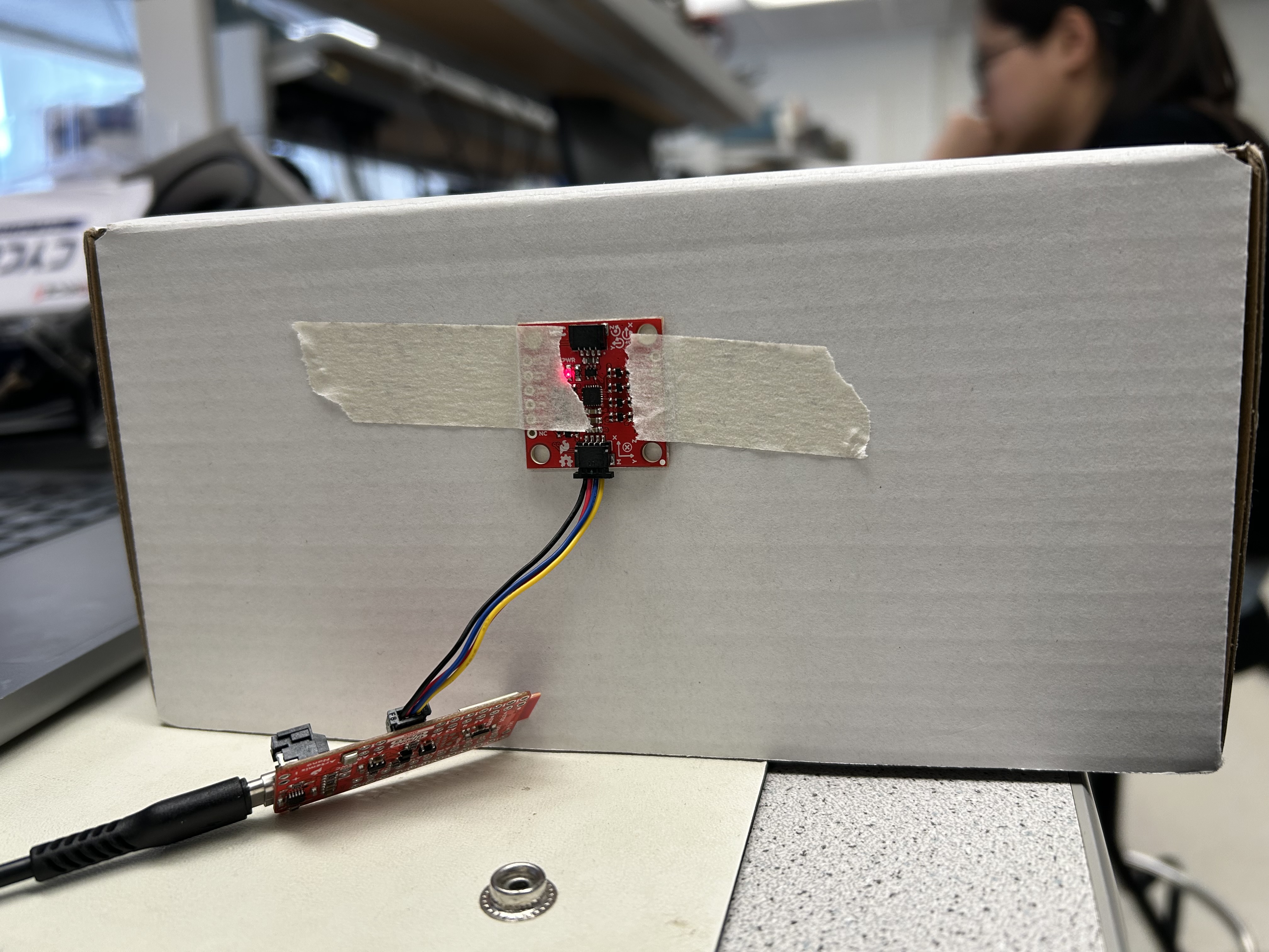 IMU Setup
After running the demo code, the IMU produced results to the serial monitor. The included video shows the data changing rapidly as I tilt the orientation of the IMU.
Significance of ADO_VAL
According to the datasheet the ADO_VAL is the LSB address of the I^2C bus. This bit allows two ICM-20948 devices to be
connected to the same I^2C bus. This value is set to 0x00 which means our device is the only one on the bus.
Accelerometer
I used the following equations to convert the accelerometer data into pitch and roll on the board.
float pitch = atan2(myICM->accY(), myICM->accZ()) * 180 / M_PI;
float roll = atan2(myICM->accX(), myICM->accZ()) * 180 / M_PI;
Using theses equations, I was able to collect 1000 data points of tilting the IMU between {-90, 0, 90} The following plot shows the result of this experiment.
Pitch
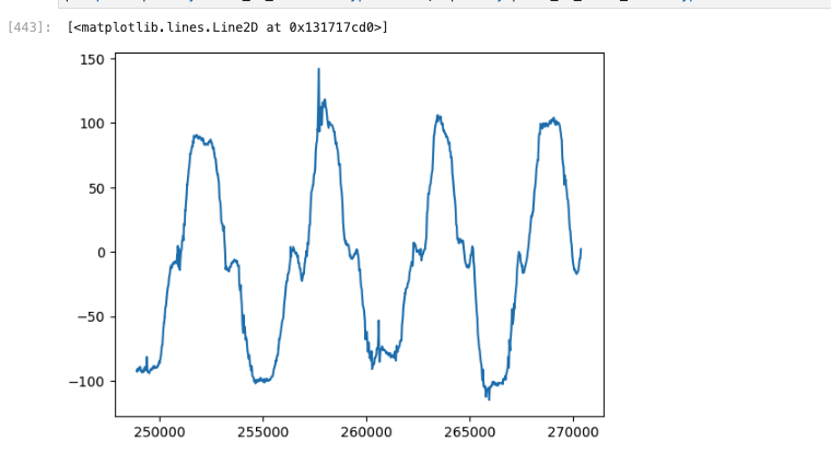
Roll
The plot shows that the data lives in the expected range but with some outliers. A good explanation for this is my jittery hand and uneven surface I used for this experiement. Sometimes, I overcompensate in the angles and go over. On first glance, the data is not very smooth, but it is still usable.
Two Point Calibration
To really investigate the accuracy of the accelerometer, I decided to use a two point calibration. To achieve this, I collected data for each of the extremes 90, 0 and -90.
The equations for the two point calibration are as follows:
actual_values = np.array([-90, 0, 90])
RawLow = np.mean(measured_values[0])
RawHigh = np.mean(measured_values[2])
ReferenceLow = actual_values[0]
ReferenceHigh = actual_values[2]
RawRange = RawHigh - RawLow
ReferenceRange = ReferenceHigh - ReferenceLow
calibrated_values = (((measured_values - RawLow) * ReferenceRange) / RawRange) +
ReferenceLow
Then for each of Pitch and Roll, I made a plot of the Ideal vs Actual values.
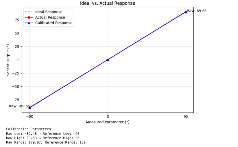
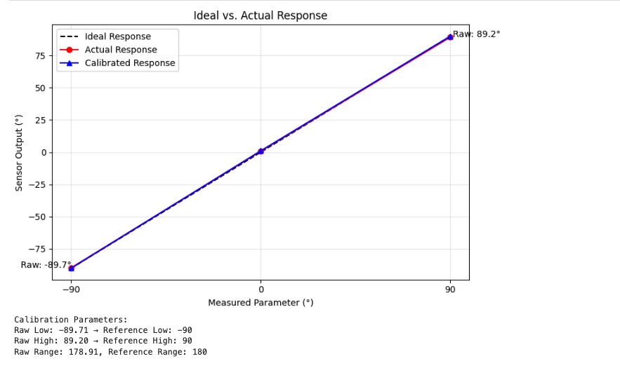
As the plot shows, the Ideal values are very close to the actual values on average. This means that the accelerometer is working accurately, and calibration is not needed.
Frequency Spectrum Analysis
Earlier, I noted that the accelerometer data is not very smooth. I used a frequency spectrum analysis to see if there was any noise in the data.
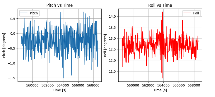
To begin, the time domain plot of the accelerometer data is shown below. The IMU was left stationary on a flat surface for this.
Then, the frequency domain plot is shown below. This was computed using the scipy fast fourier transform library. The sampling frequency is about 50Hz.
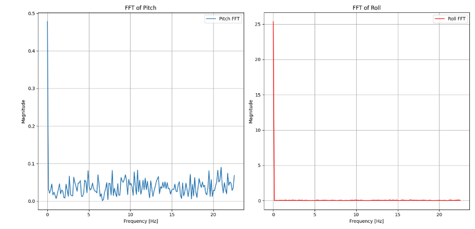
The frequency domain shows that there is noise in the data. The noise is typically absent at lower frequency but is present at higher frequencies.
To mitigate this, I designed a low pass filter with a cutoff frequency of 5Hz, a safe assumption made from the plot above.
I derived ALPHA using T/T+(2*pi*f), where T is the time period of the signal easily calculated using the sampling frequency and f is the cutoff frequency.
I used the following equations to implement the filter:
#define ALPHA 0.38
pitch_lpf = ALPHA * pitch + (1 - ALPHA) * pitch_lpf;
roll_lpf = ALPHA * roll + (1 - ALPHA) * roll_lpf;
The results of the filtering in the time domain shows that there is some attenuation in the data. The following plot shows the result of this experiment
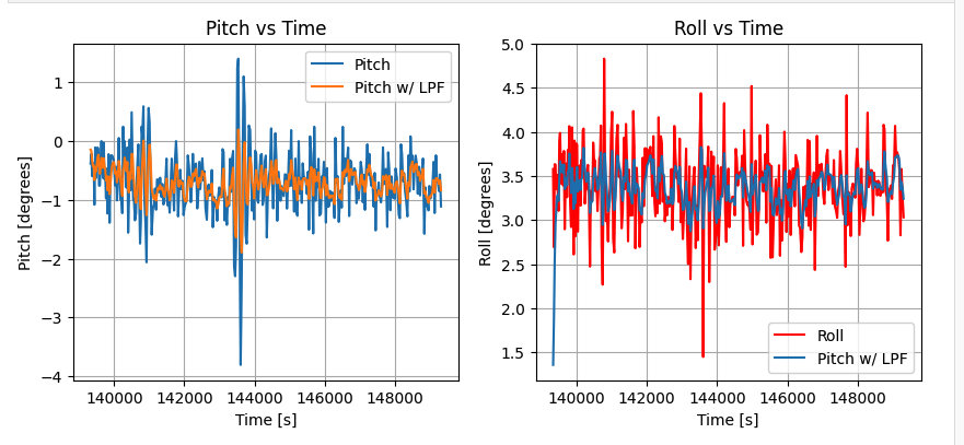
And in the frequency domain, the following plot shows the result of this experiment
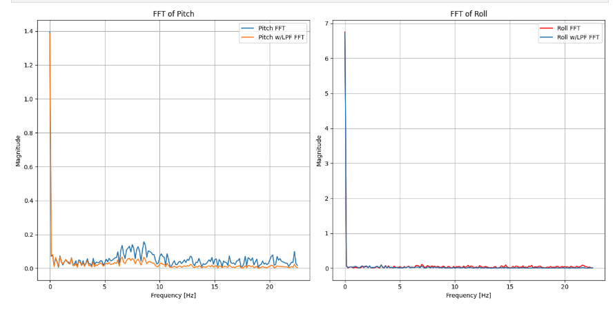
This shows that the data is much smoother now, as well as having less noise.
Gyroscope
Similarly to the the conversion done with the accelerometer, the following equations to convert the gyroscope data into pitch and roll and yaw on the board.
gy_pitch = gy_pitch + myICM->gyrY() * dt;
gy_roll = gy_roll + myICM->gyrX() * dt;
gy_yaw = gy_yaw + myICM->gyrZ() * dt;
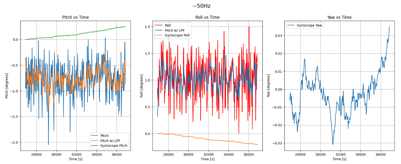
Keeping IMU stationary on a flat surface, I collected data and realized the following plot.
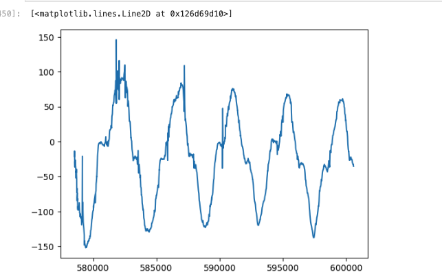
I also attempted tilting the IMU in the same way as the accelerometer. The following plot shows the result of this experiment
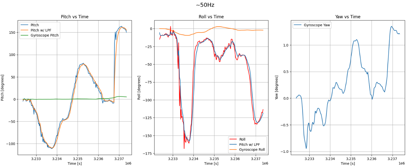
This results shows the drifting nature of the gyroscope readings. Over time, the data will drift away from the ideal values.
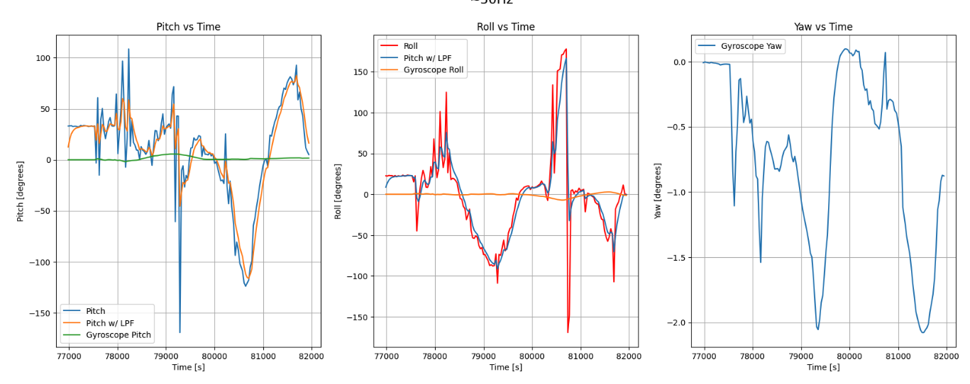
Interestingly, reducing the sampling frequency to about 30Hz casues more drift in the data as shown below.
Using sensor fusion, I designed a complimentary filter fuse the gyroscope and accelerometer data. This will help smooth out the accelerometer data and reduce the drift in the gyroscope data. The complimentary filter was designed using the following equations:
#define THETA 0.90
comp_roll = ((comp_roll + gy_roll) * (1 - THETA)) + THETA * roll;
comp_pitch = ((comp_pitch + gy_pitch) * (1 - THETA)) + THETA * pitch;
I intentionally gave more weight to the accelerometer data because it gives more accurate readings, while the gyroscope data is more stable. This checked out experiementally.
The following plot shows the result of this experiment. It highlights a comparison between the raw data from the accelerometer, the low pass filtered accelerometer data, the gyroscope data,
and finally the complimentary filter data.
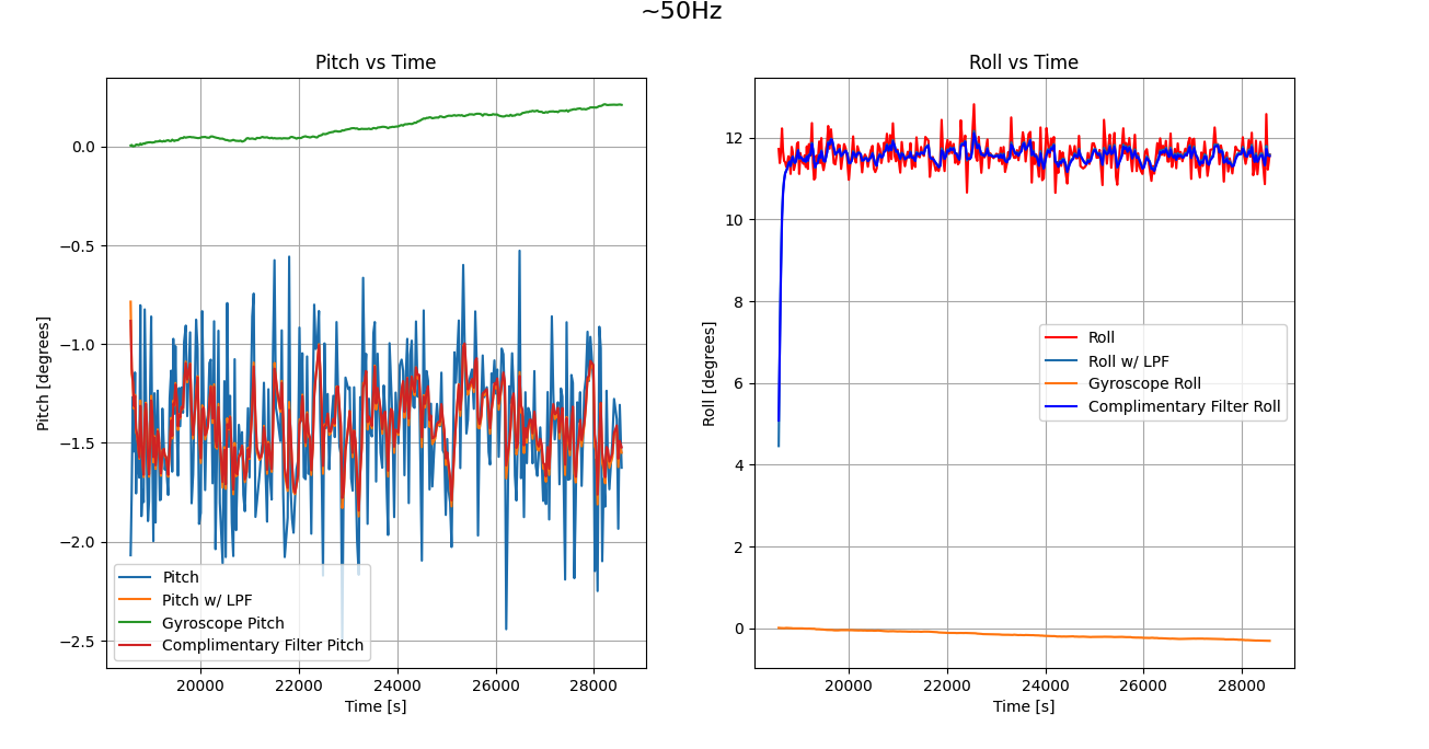
The resulting data is much smoother and less noisy. The complimentary filter results is almost identical to the Low pass filtered accelerometer data but I saw some more smoothness. For example, tapping the IMU in sharp turns showed less spikes for the complimentary filter data.
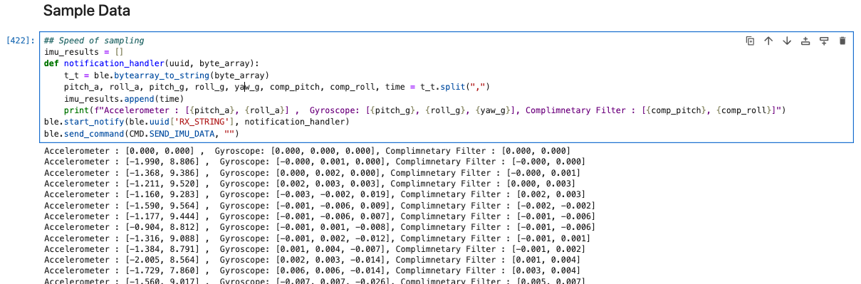
Sample Data
To determine the speed of sampling, I made sure to remove all Serial.print statements and simply record the data as soon as it is ready. My analysis involved collecting 1000 data points for each of
accelerometer, gyroscope, and complimentary filter data.
float pitch_a[DATA_ARRAY_SIZE] = { 0 };
float roll_a[DATA_ARRAY_SIZE] = { 0 };
float pitch_g[DATA_ARRAY_SIZE] = { 0 };
float roll_g[DATA_ARRAY_SIZE] = { 0 };
float yaw_g[DATA_ARRAY_SIZE] = { 0 };
float comp_pitch[DATA_ARRAY_SIZE] = { 0 };
float comp_roll[DATA_ARRAY_SIZE] = { 0 };
And in jupyter lab, I receive the data and note the time stamps.
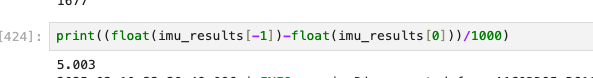
Since, I had the time stamps, I was able to calculate the difference between the first and last data points.
This worked out to be ~ 2.635 seconds. Hence, we were able to collect 1000 data points in 2.635 seconds.
Finally, instead of collecting 1000 data points, I collected data points for up to 5 seconds.
At this rate, assuming a size of 4 bytes per data point, and 8 datapoints. We store 32 bytes for each data point.
1000 data points for 5 seconds would be 32000 bytes. Since the capacity of the Artemis is 384KiB, it will take about
12,288 data points and about 61 seconds to fill up the Artemis.
int i = 1;
float dt = 0, start = millis(), last_time = start;
times[0] = start;
while ((millis() - start) < duration) {
  if (myICM->dataReady()) {
    myICM->getAGMT();
    dt = (millis() - last_time) / 1000.0;
...rest of code...
In the jupyter notebook, we can confirm that we indeed collected data points for 5 seconds.
Stunt
It was fun to see the RC car perform a stunt! The car moves really fast and was tricky to control with the included controller. Excited to see what we build with the RC car!