Kalman Filter
The purpose of this lab was to implement a Kalman Filter for the car. I was able to use the kalman filter estimate the car's position and velocity which ended up being used to supplement the ToF sensor readings.
Estimating drag and momentum
To begin the lab, I implemented a step response to to gather data on the car's position and velocity. This involved a quick method in Arduino to provide a constant pwm value to the motors for a 5 second period as it approached a wall. The following code shows a snapshot of my approach:
void step_response(unsigned long test_duration, int step_pwm,
                   unsigned long start_time) {
  unsigned long current_time = start_time;

  while ((current_time - start_time) < test_duration && curr_idx < MAX_DATA_SIZE) {
    // Apply step input
    drive_in_a_straight_line(0, step_pwm, 1.25);
    // Get sensor data
    int current_distance = distance_sensor_1.getDistance();
    // Get current timestamp
    current_time = millis();
    // Calculate velocity (change in position / change in time)
    float velocity = 0;
    float delta_time =
    (current_time - times[curr_idx - 1]) / 1000.0;  // Convert to seconds
    velocity = (current_distance - tof_vals[curr_idx - 1]) / delta_time;
    // .. code to log the data ...
}
After performing this run, I sent the data via bluetooth to my laptop to analyze and generate plots.
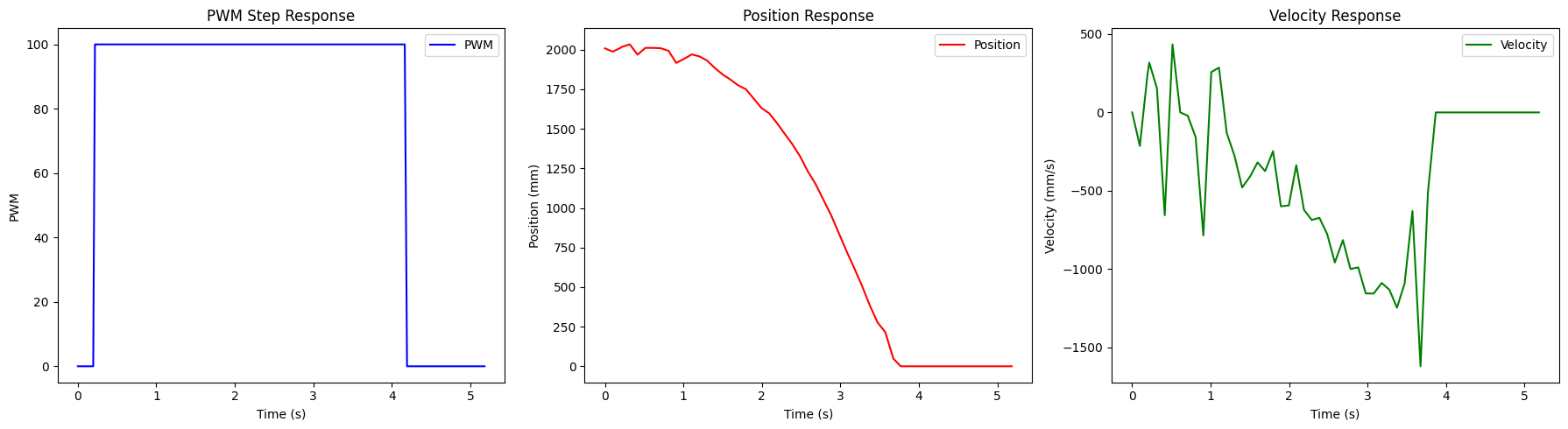 Step Response
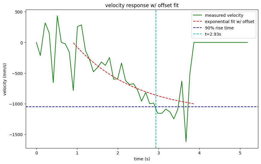
I noticed that the velocity was very noisy. I used an exponential fit to get an appromimation of the velocity so that I can determine the steady state velocity.
I then used scipy.optimize.curve_fit to fit the raw data to an exponential function. I used a cropped version of the data which clips out
the nosiy first and last couple of points. The fit was not perfect, but I got an appromimation that seemed to match an eyeball estimate of the steady state velocity.
 Velocity
The exponential fit included an offset since I clipped out the last few points. The
fit worked out to be fitted eqn: v(t) = 936.30 + -2104.71 * (1 - e^(-0.66*t))
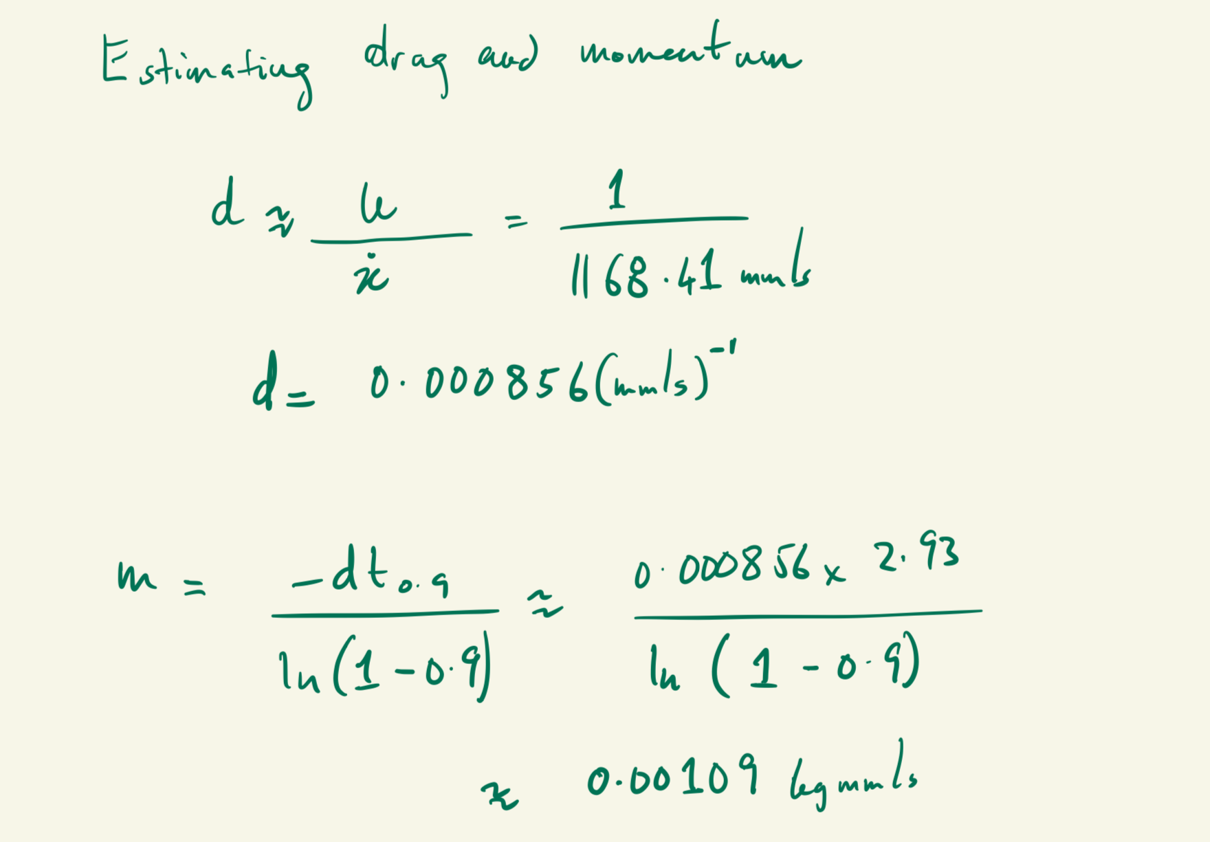
Upon obtaining the exponential relationship, it was easy to compute the steady state velocity by just observing the behavior
as time t tends to inifinity. This worked out to be 1168.41mm.s. Additionally, the 90% of rise time worked out to be 0.9*1168.41=1051.569mm/s. After obtaining
this value, I was able to use my plot to see that the 90% of the rise time happened at t=2.93s. The following equations details how I
arrived at these values:
 Eq 1.
Eq 1.
Subsequently, to obtain drag d and momentum m. I applied the state space equations:
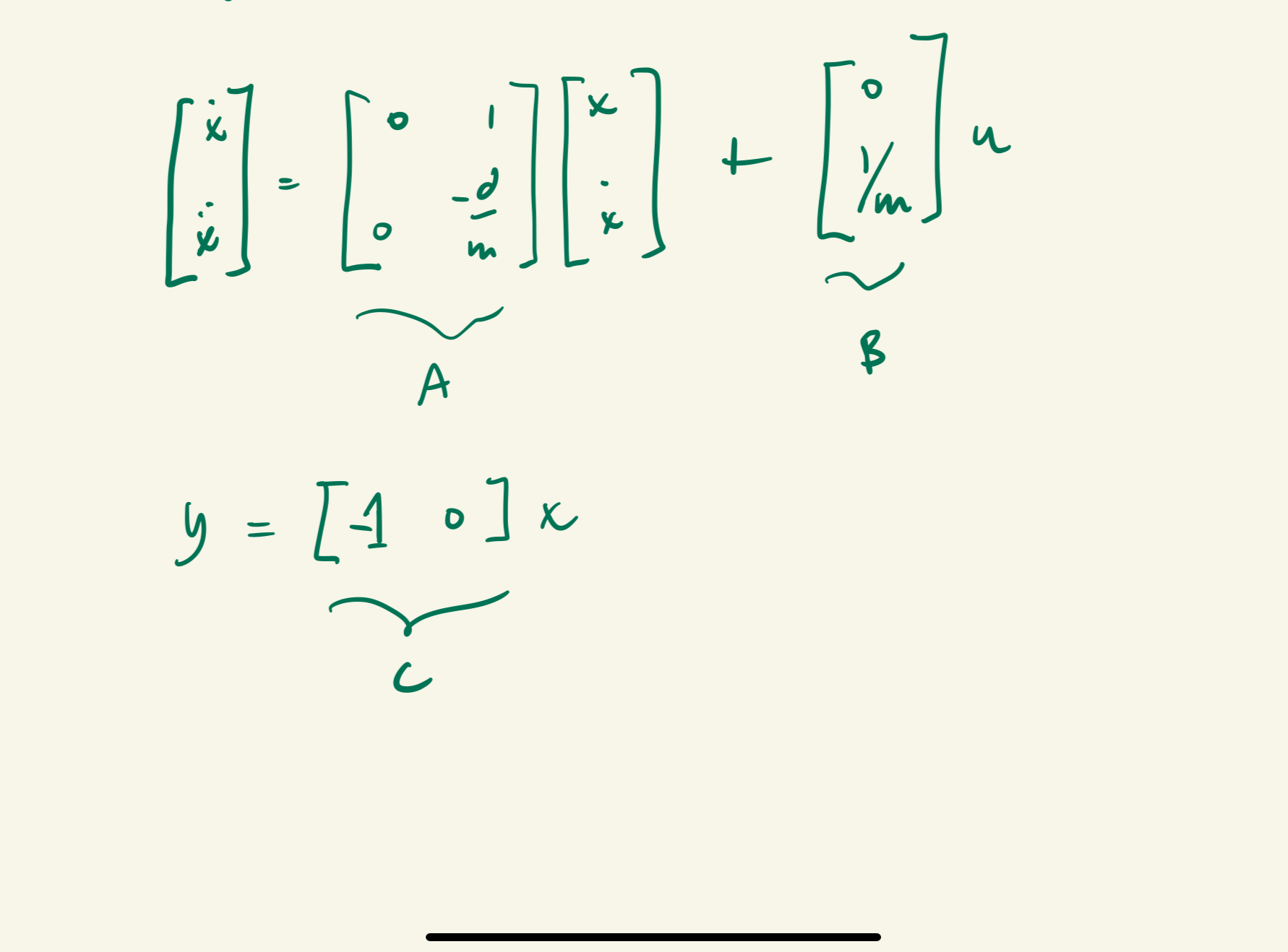 Eq 2.
Eq 2.
And the value for d was 0.000856(mm/s)^-1 and m was 0.00109kgmm/s.
 Eq 3.
Eq 3.
Initialize KF (Python)
Following the guideliens from the lab, this section was pretty straightforward.
Starting with our computed d and m, we can initialize the A and B and C matrices.
# State space
d = 0.000856
m = 0.00109
A = np.array([[0, 1], [0, -(d / m)]])
B = np.array([[0], [1 / m]])
C = np.array([[1, 0]])
Next, I used this quick method to compute the dt and then discretize the system.
# sampling time
dt = time_s[1] - time_s[0]
print(f"Sampling time: {dt:.4f} s")
This returned - Sampling time: 0.0980 s
# Discretize the system
Ad = np.eye(n) + (dt * A)
Bd = dt*B
Next, to specify the process noise and sensor noise covariance matrices. I used the method given in lectures to compute the covariance matrices using the frequency of sampling I computed earlier. I also used 20mm as the measurement noise as suggested in lecture.
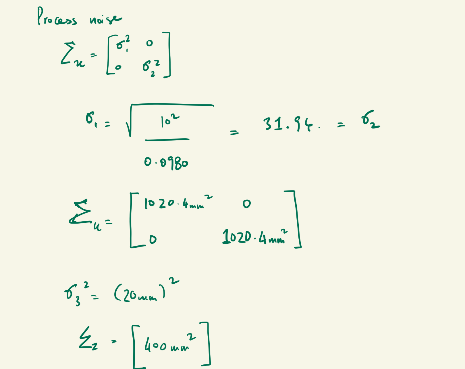 Covariance Matrices
After computing the covariance matrices, I used the following code to initialize the Kalman Filter:
X = np.array([[distance[0]], [0]])
sigma = np.array([[20**2, 0], [0, 10**2]])
sigma_1 = sigma_2 = 31.94
sigma_3 = 20
sig_u = np.array([[sigma_1**2,0],[0,sigma_2**2]])
sig_z = np.array([[sigma_3**2]])
I used an initial guess of sigma = np.array([[20**2, 0], [0, 10**2]]) as it was already experimented to be a reasonable estimate by Stephan Wagner (2024).
Finally, my code for the Kalman Filter is as follows which includes both the predict and update steps:
def kf (mu, sigma, u, y):
    mu_p = Ad.dot(mu) + Bd.dot(u)
    sigma_p = Ad.dot(sigma.dot(Ad.transpose())) + sig_u


    sigma_m = C.dot(sigma_p.dot(C.transpose())) + sig_z
    kkf_gain = sigma_p.dot(C.transpose().dot(np.linalg.inv(sigma_m)))

    y_m = y-C.dot(mu_p)
    mu = mu_p + kkf_gain.dot(y_m)
    sigma=(np.eye(2)-kkf_gain.dot(C)).dot(sigma_p)

    return mu, sigma
So we can run this filter against the data from the earlier run of the robot. I essentially iterate through the data and for each time step, run the filter. I also make sure to collect all the position data so I can plot it later.
kfs = []
uss = [1 if i==100.0 else 0 for i in pwm]
kfs.append(distance[0])
for i in range(1, len(time_s)):
    X, sigma = kf(X, sigma, uss[i], distance[i])
    kfs.append(X[0][0])
Plotting this data against the step response data, we can see that the filter is able to estimate the car's position quite well.
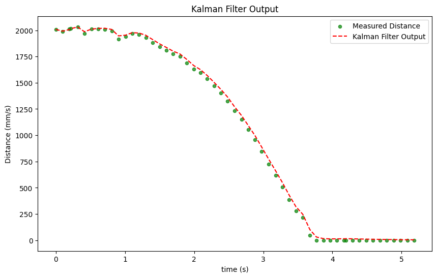 Kalman Filter
Implementing the Kalman Filter on the Robot
After verifying implementation of the Kalman Filter in Jupyter Notebook, I proceeded to implement the
filter in Arduino. This involved installing the BasicLineaAlgebra library which enable use of matrices.
As in the python code, I created variables for managing the state space matrices and the covariance matrices as well
as the A, B and C matrices.
// Kalman Filter Variables
float d = 0.000856;
float m = 0.00109;
BLA::Matrix<2, 2> A = {0, 1, 0, -d / m};
BLA::Matrix<2, 1> B = {0, 1 / m};
BLA::Matrix<1, 2> C = {1, 0};
int n = 2;
float dt = 0.0980;
BLA::Matrix<2, 2> I = {1, 0, 0, 1};
BLA::Matrix<2, 2> Ad = I + (dt * A);
BLA::Matrix<2, 1> Bd = dt * B;
float sigma_1 = 31.94;
float sigma_2 = 31.94;
float sigma_3 = 20;
BLA::Matrix<2, 2> sig_u = {sigma_1 * sigma_1, 0, 0, sigma_1 *sigma_1};
BLA::Matrix<1, 1> sig_z = {sigma_3 * sigma_3};
BLA::Matrix<2, 2> sigma = {400, 0, 0, 100};
BLA::Matrix<2, 1> mu = {0.0, 0.0};
To integrate it, I create a new function called kf_update() which will perform the update step of the kalman filter.
I chose this design because I only wanted to call this function if the time of flight actually has a reading for that
iteration of the loop. But for each iteration, I would implement the prediction step. This took the following shape:
void kf_update(BLA::Matrix<2, 1> mu_p, BLA::Matrix<2, 2> sigma_p,
               BLA::Matrix<2, 1> &mu, BLA::Matrix<2, 2> &sigma, int distance) {

  BLA::Matrix<1, 1> sigma_m = (C * (sigma_p * (~C))) + sig_z;
  float sigma_m_inv = 1.0f / sigma_m(0, 0);
  BLA::Matrix<2, 1> kkf_gain = sigma_p * ((~C) * sigma_m_inv);

  BLA::Matrix<1, 1> y = {(float)distance};
  BLA::Matrix<1, 1> y_m = y - (C * mu_p);
  mu = mu_p + (kkf_gain * y_m);
  sigma = (I - (kkf_gain * C)) * sigma_p;
}
And in the main loop, I call this function as follows:
void loop() {
    if (is_pid_running) {
      distance_sensor_1.startRanging();
      // Always run Kalman Filter prediction
      float scaled_p = (float)last_pwm / 100.0f;
      BLA::Matrix<2, 1> mu_p = (Ad * mu) + (Bd * scaled_p);
      BLA::Matrix<2, 2> sigma_p = (Ad * (sigma * ~Ad)) + sig_u;

      if (distance_sensor_1.checkForDataReady()) {
        int raw_distance = distance_sensor_1.getDistance();
        distance_sensor_1.clearInterrupt();
        distance_sensor_1.stopRanging();

        // Update Kalman Filter since we have new data
        kf_update(mu_p, sigma_p, mu, sigma, raw_distance);
        current_distance = raw_distance;
      }

      float estim_dist = mu(0, 0);

      last_pwm = pid_control(estim_dist);

      // Log the data
      if (curr_idx < MAX_DATA_SIZE) {
        times[curr_idx] = (float)millis();
        pwm_vals[curr_idx] = last_pwm;
        tof_vals[curr_idx] = current_distance;
        predicted_kalman_vals[curr_idx] = estim_dist;
        curr_idx++;
      }

      // ...code to drive motors with scaled PWM and proper direction
  }
  }
}
NOTE: mu is initialized in a init_pid() function which is called when the START_PID command is received.
void init_pid() {
  accumulated_error = 0.0;  // Reset integral term
  last_pid_time = millis(); // Reset time
  last_pwm = 0;

  // Initialize the kalman filter state
  distance_sensor_1.startRanging();
  while (!distance_sensor_1.checkForDataReady()) {
    delay(1);
  }
  current_distance = distance_sensor_1.getDistance();
  distance_sensor_1.clearInterrupt();
  distance_sensor_1.stopRanging();

 // Initialize the Kalman filter state
  mu = {(float)current_distance, 0.0};
  is_pid_running = true;
  curr_idx = 0;
}
Once the Kalman Filter was already set up, I ran it on the robot car and made a few runs towards the wall to see how it performed.
I started with a run where gains were 0.08|0.0005|1.0 (kp, ki and kd respectively). The video below is the result of this run.
And below is a plot of the data collected from this run.
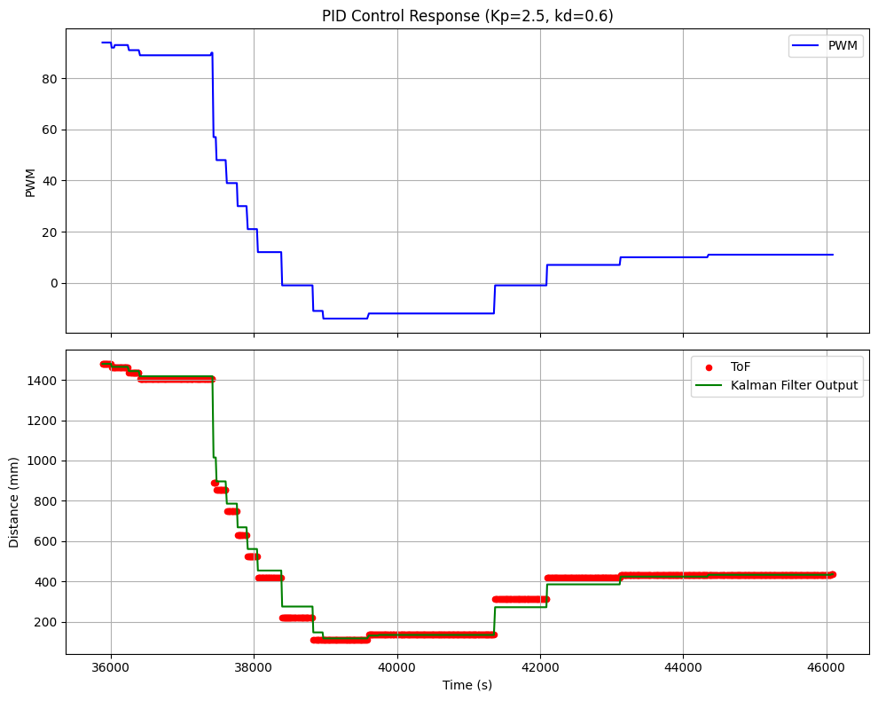 Kalman Filter 0.08|0.0005|1.0
It was clear from the plot and video that the kalman filter was working. In the plot, we can see the kalman filter estimate the car's position when the time of flight didn't give any readings. However, the car was initially overshooting the setpoint and correcting itself. This was good but I gave it another try which a smaller kp gain of 0.06 so that it can slowly approach the setpoint.
The resulting run is shown below.
And below is a plot of the data collected from this run. The approach to the setpoint was much smoother although I sacrificed some speed of approach. At this point, I was confident my kalman filter was working.
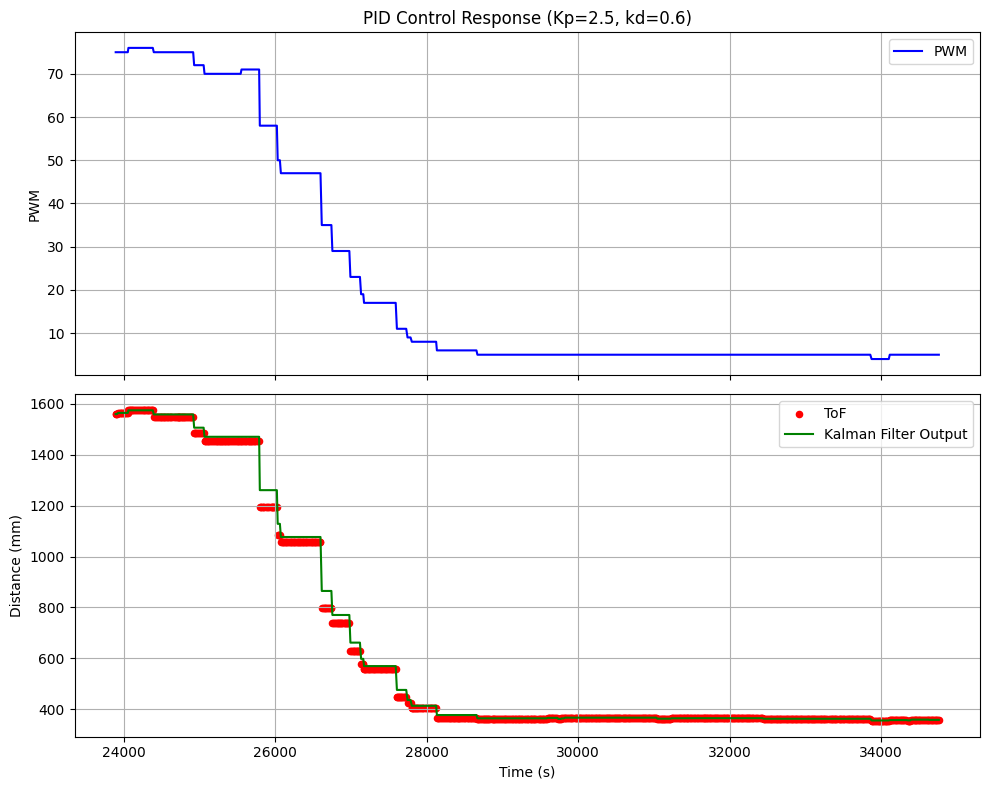 Kalman Filter 0.06
Conclusion
This was a very fun lab to implement a kalman filter on the robot car. I was able to use the kalman filter to estimate the car's position and velocity which ended up being used to supplement the ToF sensor readings. I also learned a lot about the kalman filters work in general [1]Many thanks to Stephan Wagner (2024)