Linear PID control and Linear interpolation
The purpose of the lab was to implement a PID controller with linear Interpolation for the RC car driving towards a wall and stopping precisely 304 mm away from the wall.
Prelab
It was important to establish a robust debugging and data acquisition infrastructure. I implemented the BLE communication between the Artemis and my computer so I can send commands, control the car, and also receive data from the car. The system operated as follows:
Commands
The robot responds to BLE commands such as START_PID (initiate PID control), STOP_PID (stop the robot), SET_PID_GAINS (set kp, ki and kd), and most importantly SEND_PID_DATA. After
a control run, the python script will be able to receive the data accumulated over that run and plot it using matplotlib. This allows for immediate visualization of controller
performance and was paramount for debugging. The data I collected for each run includes: the timestamp, the reading from the time of flight sensor, and the pwm values for that run. The following code shows how
I accumulated this data.
  BLEDevice central = BLE.central();
  while (central.connected()) {
    if (rx_characteristic_string.written()) {
      handle_command(); // Parse and execute BLE command
    }
    // ... code to read sensors and calculate PID values ...
    if (is_pid_running) {
      // ... sensor readings, PID calculation, pwm output ...
      if (curr_idx < MAX_DATA_SIZE) { // Store data for debugging
        times[curr_idx] = (float)millis();
        tof_vals[curr_idx] = dist;
        pwm_vals[curr_idx] = pwm;
        curr_idx++;
      }
    }
  }
Operation
The general approach is as follows. Upon receiving the START_PID command, the code set is_pid_running to true and begins the PID control, logging data to the arrays. The arrays have a max
capacity of MAX_DATA_SIZE. I didn't expect this to fill up after seeing the result from open loop control. Once this is set, the artemis loop simply repeatedly collects time of flight reading and calculates the PID values to generate PWM values.
I then use these PWM values to control the motors using methods I implemented in the last lab. These include drive_in_a_straight_line, which gives the wheels forward or reverse pwm depending on the arguments to the function. Below is the
code snippet to illustrate this. The START_PID and STOP_PID commands are handled in the handle_command which is called in the main loop on every iteration.
case START_PID:
    is_pid_running = true;
    distance_sensor_1.startRanging(); // Start continuous ranging
    break;
case STOP_PID:
    is_pid_running = false;
    distance_sensor_1.stopRanging();
    stop();
    break;
while (central.connected()) {
    if (rx_characteristic_string.written()) {
      handle_command();
    }

    if (is_pid_running) {
      distance_sensor_1.startRanging();
      int pwm;
      if (distance_sensor_1.checkForDataReady()) {
        int dist = distance_sensor_1.getDistance();
        distance_sensor_1.clearInterrupt();
        distance_sensor_1.stopRanging();

        pwm = pid_control(dist); // calculate pwm based on distance to target

        // ...code to log the data ...
      }


      // Drive motors with scaled PWM and proper direction
      if (abs(pwm) > 0) {
        // Scale PWM to avoid deadband
        int scaled_pwm;
        if (pwm > 0) {
          scaled_pwm = map(pwm, 0, 255, 40, 255);
          drive_in_a_straight_line(1, scaled_pwm, 1.25); // forward
        } else {
          scaled_pwm = map(abs(pwm), 0, 255, 40, 255);
          drive_in_a_straight_line(0, scaled_pwm, 1.25); // backward
        }
      } else {
        stop(); // When PWM is exactly 0
      }
    }
  }
Finally, I included a kill-switch in case the bluetooth connection is lost. This happens in the loop
  while (central.connected()) {
    // .. code to read sensors and calculate PID values ...
  }

  // if bluetooth connection is lost, stop the car
  distance_sensor_1.stopRanging();
  distance_sensor_2.stopRanging();
  stop();
As with previous labs, my python script mostly included ble notification handlers and sends commands to the artemis. For example, here is how I collect the data sent after a run:
results = []

def notification_handler(uuid, byte_array):
    time, tof, pwm = ble.bytearray_to_string(byte_array).split('|')
    results.append([float(time), int(tof), int(pwm)])

ble.start_notify(ble.uuid['RX_STRING'], notification_handler)
ble.send_command(CMD.SEND_PID_DATA, "")
Lab Tasks
For the control task, I opted to begin with only Proportional (P) controller. Given the objective of moving towards a wall and stopping at a precise distance, a P- controller seemed straightforward and an intuitive starting point since I can simply adjust the motor output proportionally to the error. The error is defined as the difference between the desired distance (setpoint: 304mm) and the measured distance recorded by the ToF sensor.
I began by configuring the time of flight sensor to a long distance mode. This is because it is the only mode that can give reading between 1-4ft. However, I made sure to set the timing budget to 20ms. This is the minimum timing budget that can be used for the long distance mode. And it is necessary to have a fast enough timing budget to ensure that we can have a faster response and consequently more accurate control of the car.
I added some Serial.print statements to my code to get an idea of the ToF rate and the PID rate. The ToF rate was ranging between 27-35Hz. While the PID loop
was ranging between 104-150Hz. The bottle neck is the ToF sensor. To improve on this, I added a linear extrapolator that will try to guess the distance if the
ToF sensor is not giving a reading. See section Linear Interpolation
 Linear Interpolation
The following code highlights the core of the PID control algorithm using only kp
int pid_control(int curr_distance) {

  int error = pid_position_target - curr_distance;

  // Proportional controller
  float pwm = kp * error;

  if (pwm > 0 && pwm > 255) {
    pwm = 255;
  }
  return pwm;
}
I simply calculate the error between the setpoint and the current distance. Then, I multiply the error by the kp gain and use that result to set
the output pwm. I also made sure to cap the pwm output for the car to not exceed the max pwm value of 255. The value of kp is set by the bluetooth command SET_PID_GAINS.
Also, from lab4 I found a deadband for my motor. It was only able to overcome friction at about 40 pwm. So I scaled the pwm output of the controller using the arduino map function
// Drive motors with scaled PWM and proper direction
if (abs(pwm) > 0) {
  // Scale PWM to avoid deadband
  int scaled_pwm;
  if (pwm > 0) {
    scaled_pwm = map(pwm, 0, 255, 40, 255);
    drive_in_a_straight_line(1, scaled_pwm, 1.25); // forward
  } else {
    scaled_pwm = map(abs(pwm), 0, 255, 40, 255);
    drive_in_a_straight_line(0, scaled_pwm, 1.25); // backward
  }
} else {
  stop(); // When PWM is exactly 0
}
I began testing with a Kp=0.08. I made this guess based on previous years. I notice that the car moves fast, however it only stabilizes at about 200mm (-104 mm error).
Essentially, there is fast response but it doesn't reach the setpoint, and the there is a steady state error. It approaches the setpoint aggressively and also makes large corrections.
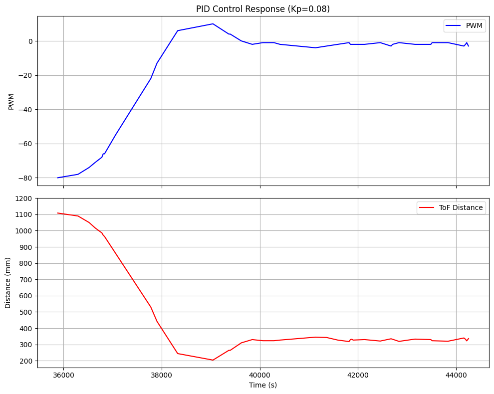 PID Control kp=0.08
And the following video shows the result of this experiment.
I wasn't satisfied with this result. So I attempted to tune the kp parameter. A pattern started to emerge. As the following plots show for kp=0.07 and kp=0.05, lower values keep much slower responses but there is still
a steady state error appearing in the oscillations. This is a sign that I needed to correct this error with an integrator term.
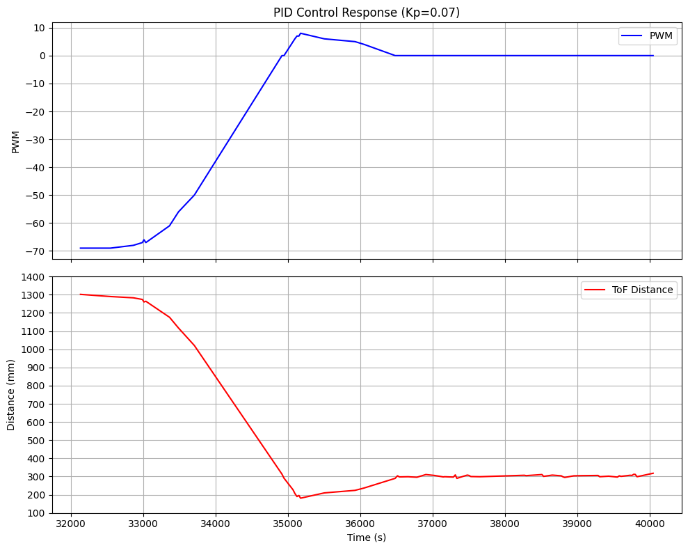 PID Control kp=0.07
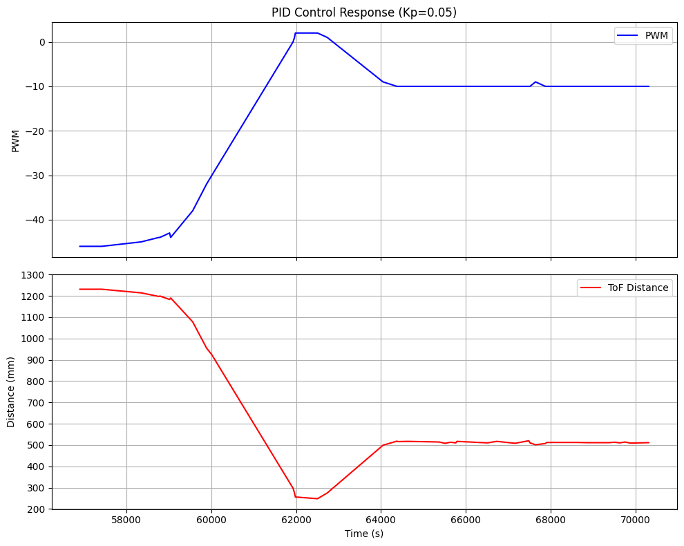 PID Control kp=0.05
To add an integrator term, I simply updated my pid_control() method as follows:
//.. existing code ..
unsigned long current_time = millis();
float dt =
  (float)(current_time - last_pid_time) / 1000.0;  // Convert ms to seconds
last_pid_time = current_time;

if (dt > 0) {
  accumulated_error += error * dt;
}

// Calculate P and I terms
float p_term = kp * error;
float i_term = ki * accumulated_error;
if (i_term > 200) {
  i_term = 200;
} else if (i_term < -200) {
  i_term = -200;
}
float pwm = p_term + i_term;
I basically use the time between the last PID calculation and this to multiply the accumulated error. I also capped the I term to prevent it from going over 200 or below -200. This is an idea I got from Nila Narayan's (2024) lab.
Fortunately, my python script already had provision for me to change the pid gains without having to
recompile the code to the Artemis. I simply updated the SET_PID_GAINS command to accept a new kp and ki value.
Upon testing multiple values, and using the lab handout as guide, I figured I could choose a slower and conservative controller or a more aggressive one. I knew
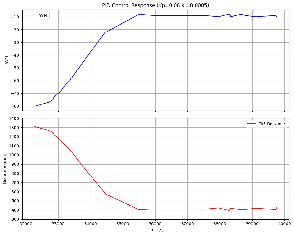
I wanted a faster controller but also one that didn't prove difficult to tune. I ended up choosing kp=0.08 and ki=0.005 which gave me a much smoother response.
The following plot shows the result of this experiment. Once the car slightly passes the setpoint, it doesn't overcorrect or undercorrect,
it simply glides to the setpoint.
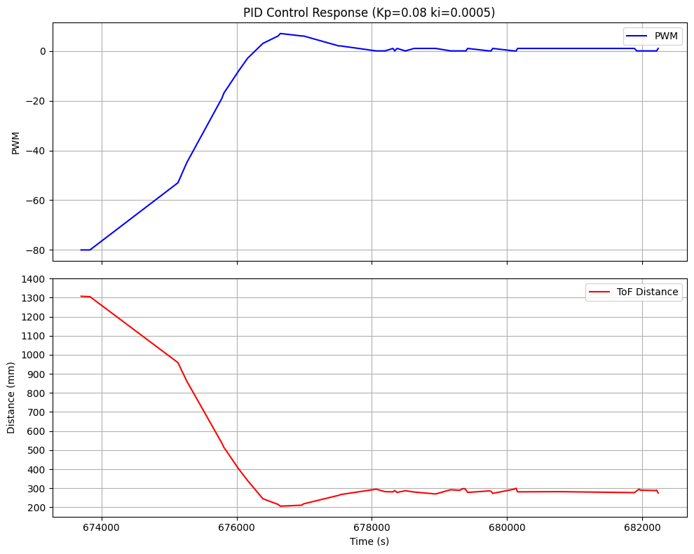 PID Control kp=0.08
At this point, I was confident with my results. The following video shows the result of this experiment. The car approaches the setpoint relatively quickly but can still correct its speed to meet the setpoint.
Linear Interpolation
Linear extrapolation aims to predict the future distance to the wall based on recent TOF sensor readings. This is valuable for us because it decouples the PID control loop frequency from the TOF sensor update rate. This means we can still proceed to get distance readings even if the TOF sensor is not giving us a reading quickly enough.
To achieve this, I added a new function called extrapolate_distance() which calculates the next distance based on the amount of time since the last reading and the slope
of the last two datapoints. The following code shows how I calculate this.
int extrapolate_distance() {
  if (last_tof_time == 0 || second_last_tof_time == 0) {
    return last_tof_reading;
  }

  float time_diff = last_tof_time - second_last_tof_time;
  if (time_diff == 0)
    return last_tof_reading;

  float slope = (last_tof_reading - second_last_tof_reading) / time_diff;

  unsigned long current_time = millis();
  float time_since_last = current_time - last_tof_time;

  float estimated_distance = last_tof_reading + (slope * time_since_last);

  return (int)estimated_distance;
}
Then I simply add this to the main pid loop. If the condition that checks if the sensor is ready fails, we extrapolate the data
if (is_pid_running) {

  distance_sensor_1.startRanging();
  int pwm;
  if (distance_sensor_1.checkForDataReady()) {
    int dist = distance_sensor_1.getDistance();
    distance_sensor_1.clearInterrupt();
    distance_sensor_1.stopRanging();

    // Update history
    second_last_tof_reading = last_tof_reading;
    second_last_tof_time = last_tof_time;
    last_tof_reading = dist;
    last_tof_time = millis();

    pwm = pid_control(dist);

    // ...code to log the data
  } else {
    int estimated_dist = extrapolate_distance();
    pwm = pid_control(estimated_dist);
  }

  // ...code to drive motors with scaled PWM and proper direction
}
This resulted in a better result, helping the car to make less oscillations. The approach is much sharper at the setpoint. No need to overcorrect or undercorrect. However, the data is slightly less accurate. A more powerful extrapolation algorithm like a Kalman filter would be better suited for this.
 PID Control with Extrapolation
Conclusion
This lab demonstrated the effective implementation of PID control on our robot car, starting with a simple P-controller (kp=0.08) that showed quick but oscillatory behavior, and evolving to a PI-controller (kp=0.08, ki=0.005) that achieved smoother, more accurate positioning. The addition of linear extrapolation helped overcome the ToF sensor's limited update rate (27-35Hz), resulting in better control performance. While successful, this implementation revealed opportunities for future improvements, particularly in exploring more sophisticated state estimation techniques like Kalman filtering.