Localization
The purpose of this lab was to implement and test a grid-based localization algorithm using a Bayes Filter within a simulated environment. The goal was to estimate the robot's pose (x, y, θ) over time by probabilistically using noisy odometry data and simulated sensor measurements.
Setup: Understanding Grid Localization and Bayes Filter
Before diving into the implementation, it was essential to understand the core concepts.
Grid Localization: Since the robot's possible pose (x, y, θ) exists in a continuous space, tracking its exact position is computationally intractable. Grid localization simplifies this by discretizing the environment into a finite 3D grid. Each cell in this grid represents a possible discrete pose (a range of x, y, and θ values). Instead of tracking an exact pose, we track the probability that the robot is located within each grid cell. This probability distribution across all cells is called the belief. In this lab, the grid had dimensions (12, 9, 18) corresponding to discretized x, y, and orientation axes.
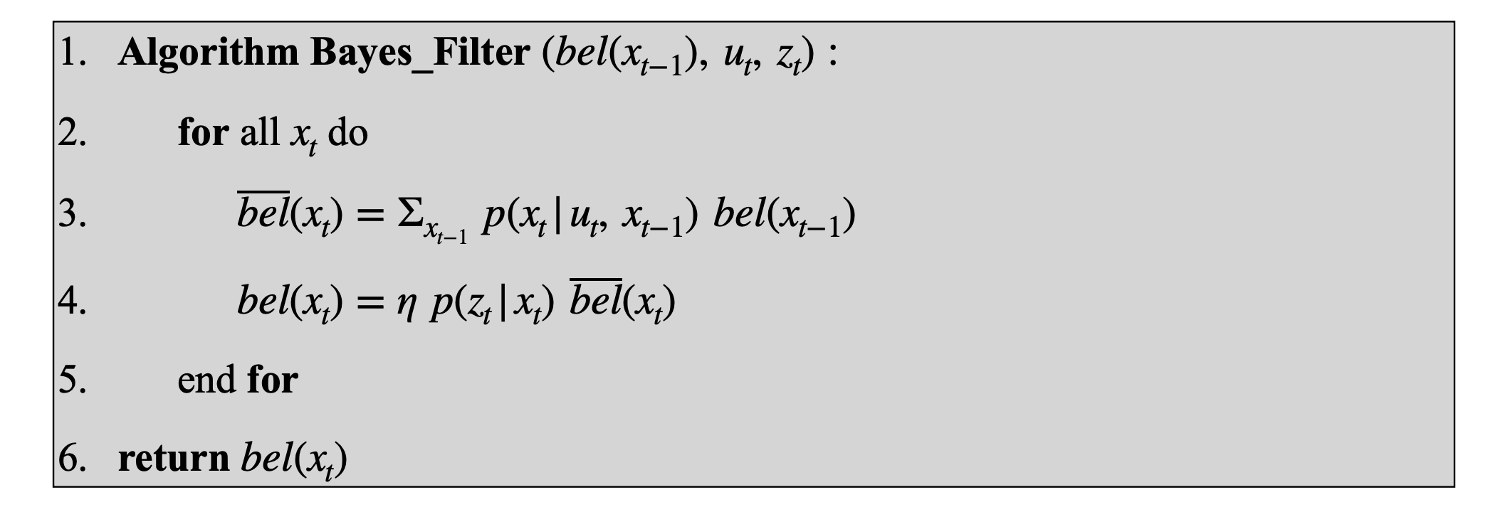
Bayes Filter: The Bayes Filter is a recursive algorithm used to estimate the state of a system (in our case, the robot's pose) as it evolves over time. It operates in a two-step cycle:
- Prediction: Uses the previous belief state and a motion model (incorporating control inputs) to predict the current belief state. This step generally increases uncertainty due to motion noise.
- Update: Incorporates sensor measurements using a sensor model to update the predicted belief by correlating sensor readings with the known map
 Bayes Algorithm
Lab Tasks: Implementing the Bayes Filter
The core task was to implement the prediction and update steps within the provided simulator framework. This involved implementing several key functions.
1. Computing Control Input (compute_control)
Since our odometry motion model requires control inputs in the form of (rotation1, translation, rotation2), this function calculates these values based on the difference between the odometry poses from one time-step ago and this timestep (prev_pose and cur_pose).
def compute_control(cur_pose, prev_pose):
    """ Given the current and previous odometry poses, this function extracts
    the control information based on the odometry motion model.

    Args:
        cur_pose  ([Pose]): Current Pose
        prev_pose ([Pose]): Previous Pose

    Returns:
        [delta_rot_1]: Rotation 1  (degrees)
        [delta_trans]: Translation (meters)
        [delta_rot_2]: Rotation 2  (degrees)
    """
    cur_x, cur_y, cur_theta = cur_pose
    prev_x, prev_y, prev_theta = prev_pose

    # calculate rot1
    delta_rot_1 = mapper.normalize_angle(
        np.degrees(np.arctan2(cur_y - prev_y, cur_x - prev_x)) - prev_theta,
    )

    # Calculate the translation distance
    delta_trans = np.hypot(cur_y - prev_y, cur_x - prev_x) # Efficiently computes sqrt((x2-x1)**2 + (y2-y1)**2)

    # Calculate the final rotation relative to the direction of movement
    delta_rot_2 = mapper.normalize_angle(cur_theta - prev_theta - delta_rot_1)
    return delta_rot_1, delta_trans, delta_rot_2
This implementation uses np.arctan2 for angle calculation, np.hypot (hypotenuse) for efficient distance calculation, and mapper.normalize_angle to ensure all angles are wrapped correctly within the [-180, 180) degree range.
2. Odometry Motion Model (odom_motion_model)
This function calculates the probability of transitioning from prev_pose to cur_pose given a control input u = (rot1, trans, rot2), i.e., p(cur_pose | prev_pose, u). It uses the compute_control function to find the hypothetical control (delta_rot_1, delta_trans, delta_rot_2) required for this specific transition and compares it to the actual measured control input u. The comparison uses Gaussian distributions to model noise in rotation and translation.
def odom_motion_model(cur_pose, prev_pose, u):
    """ Odometry Motion Model

    Args:
        cur_pose  ([Pose]): Current Pose
        prev_pose ([Pose]): Previous Pose
        u (rot1, trans, rot2) (float, float, float): A tuple with actual measured control data

    Returns:
        prob [float]: Probability p(x'|x, u)
    """
    # Calculate the control required for this specific hypothetical transition
    delta_rot_1, delta_trans, delta_rot_2 = compute_control(
        cur_pose, prev_pose)

    # Calculate probability of each component based on Gaussian noise model
    prob_rot_1 = loc.gaussian(delta_rot_1, u[0], loc.odom_rot_sigma)
    prob_trans = loc.gaussian(delta_trans, u[1], loc.odom_trans_sigma)
    prob_rot_2 = loc.gaussian(delta_rot_2, u[2], loc.odom_rot_sigma)

    # Total probability is the product
    return prob_rot_1 * prob_trans * prob_rot_2
This function relies on the loc.gaussian helper function and predefined noise sigmas (loc.odom_rot_sigma, loc.odom_trans_sigma).
3. Prediction Step (prediction_step)
This is the core of the Bayes Filter's prediction phase. It computes the predicted belief (loc.bel_bar) based on the previous belief (loc.bel) and the measured odometry change (cur_odom, prev_odom). It iterates through all possible previous states x and current states x', summing the probability contributions: bel_bar(x') = Σ [ p(x' | x, u) * bel(x) ].
def prediction_step(cur_odom, prev_odom):
    """ Prediction step of the Bayes Filter.
    Update the probabilities in loc.bel_bar based on loc.bel from the previous time step and the odometry motion model.

    Args:
        cur_odom  ([Pose]): Current Pose from odometry
        prev_odom ([Pose]): Previous Pose from odometry
    """
    u = compute_control(cur_odom, prev_odom)
    loc.bel_bar = np.zeros_like(loc.bel)

    # numpy for efficient iteration
    # Get indices of all possible current states (x')
    grid_x, grid_y, grid_t = np.indices(loc.bel.shape)
    flat_grid_x = grid_x.ravel()
    flat_grid_y = grid_y.ravel()
    flat_grid_t = grid_t.ravel()

    # only iterate through previous states (x) with non-negligible probability
    threshold = 1e-4
    prev_poses_indices = np.argwhere(loc.bel >= threshold)

    for px, py, pt in prev_poses_indices:
        prev_state_coords = mapper.from_map(px, py, pt)
        prev_belief_weight = loc.bel[px, py, pt]

        # Calculate transition probabilities p(x'|x, u) for all possible current states x'
        # Uses np.fromiter for potentially faster iteration than a Python loop
        p_trans_flat = np.fromiter(
            (odom_motion_model(mapper.from_map(cx, cy, ct), prev_state_coords, u) # Calculate p(x'|x, u) for each x'=(cx,cy,ct)
             for cx, cy, ct in zip(flat_grid_x, flat_grid_y, flat_grid_t)),
            dtype=float,
            count=flat_grid_x.size,
        )
        p_trans = p_trans_flat.reshape(loc.bel.shape) # Reshape back to grid dimensions

        # Add weighted contribution to the predicted belief: bel(x) * p(x'|x, u)
        loc.bel_bar += prev_belief_weight * p_trans

    # Normalize the predicted belief to sum to 1
    loc.bel_bar /= np.sum(loc.bel_bar)
To optimize this potentially slow function I implemented two key strategies leveraging NumPy:
- Thresholding: Instead of looping through all possible previous states, np.argwhere(loc.bel >= threshold) selects only those grid cells where the previous belief loc.bel was higher than the threshoold. This significantly reduces the number of outer loop iterations.
- Vectorized Calculation: While the outer loop iterates through probable previous states, the calculation of transition probabilities p(x'|x, u) for all possible current states x' is done efficiently using np.fromiter. This avoids a nested Python loop over current states, leveraging NumPy's speed for the inner computation. np.indices and .ravel() are also used to generate the coordinates for all current states efficiently.
4. Sensor Model (sensor_model)
This function calculates the likelihood of observing the actual sensor readings by using an array of observations and calculates the probabilities of each of these occurring for the current state as a Gaussian distribution and a provided standard deviation .
def sensor_model(obs):
    """ Calculates the likelihood p(z_k|x) for each individual sensor beam k.

    Args:
        obs ([ndarray]): A 1D array (size 18) of EXPECTED sensor readings for a specific pose x.

    Returns:
        [list]: Returns a list (size 18) of likelihoods p(z_k|x) for each measurement k=1..18.
    """
    # Compare each expected reading obs[i] with the actual reading loc.obs_range_data[i]
    return [loc.gaussian(obs[i], loc.obs_range_data[i], loc.sensor_sigma)
            for i in range(mapper.OBS_PER_CELL)]
5. Update Step (update_step)
This function performs the second phase of the Bayes Filter. It updates the predicted belief (loc.bel_bar) using the sensor model likelihood to produce the final belief (loc.bel). The update rule is: bel(x) = η * p(z | x) * bel_bar(x) where p(z | x) is the likelihood of observing the entire measurement set z given pose x.
def update_step():
    """ Update step of the Bayes Filter.
    Update the probabilities in loc.bel based on loc.bel_bar and the sensor model likelihood p(z|x).
    """
    # Get indices of all possible current states (x)
    grid_x, grid_y, grid_t = np.indices(loc.bel.shape)
    flat_grid_x = grid_x.ravel()
    flat_grid_y = grid_y.ravel()
    flat_grid_t = grid_t.ravel()

    # Uses np.fromiter for potentially faster iteration
    p_likelihood_flat = np.fromiter(
            (
                # Calculate product Π p(z_k|x) for the state (x, y, t)
                np.prod( # Product rule for independent sensors
                    sensor_model( # Get list of p(z_k|x) for this state
                        mapper.get_views(x, y, t) # Get expected observations for this state
                    )
                )
                for x, y, t in zip(flat_grid_x, flat_grid_y, flat_grid_t) # Iterate through all states x
            ),
            dtype=float,
            count=flat_grid_x.size,
        )
    p_likelihood = p_likelihood_flat.reshape(loc.bel.shape) # Reshape likelihood grid

    # Apply Bayes update rule: bel(x) = p(z|x) * bel_bar(x)
    loc.bel = p_likelihood * loc.bel_bar

    loc.bel /= loc.bel.sum()
Similar to the prediction step, this implementation leverages NumPy for faster computation.
Simulation Results
I ran the simulation using the implemented Bayes Filter along the predefined trajectory. The simulator plotted the estimated pose (highest probability cell)(in blue), the ground truth (in green), and the raw odometry(in red). To highlight the effectiveness of the Bayes Filter, I compared the results of the pure odometry trajectory and the bayes filter trajecttory. The following videos show this.
Raw Odometry
Bayes Filter Localization
As expected, the pure odometry trajectory quickly diverged from the ground truth due to the accumulation of noise. The Bayes Filter, however, was able to significantly mitigate this. By incorporating sensor measurements in the update step, the filter could correlate the observed distances with the known map, effectively "pulling" the estimated pose back towards the true location whenever the belief became too uncertain or drifted too far.
Conclusion
This lab provided practical experience in implementing a Bayes Filter, in a grid-based representation. Key takeaways include:
- Understanding the prediction (motion model) and update (sensor model) steps is crucial.
- Discretizing the state space makes the problem tractable but introduces approximation.
- Careful handling of angles (normalization) is necessary.
- Fusing noisy odometry with sensor measurements drastically improves localization accuracy compared to using odometry alone.
- Optimization techniques, particularly leveraging NumPy for vectorized operations and avoiding unnecessary computations (like thresholding low-probability states), are vital for achieving reasonable performance, especially in Python.
- The successful implementation in the simulator demonstrates the power of probabilistic methods for robust robot localization in the presence of noise and uncertainty. Excited to see it work on the actual robot in the next lab