Real-World Localization

Author: Akinfolami Akin-Alamu

The purpose of this lab was to apply the Bayes Filter localization algorithm developed in simulation (Lab 10) to the actual physical robot. A key difference and simplification for this lab was to rely only on the sensor update step, omitting the motion model prediction step, due to the anticipated high level of noise in the real robot's odometry. The goal was to localize the robot starting from a uniform belief (no prior knowledge of position) using a single 360-degree sensor scan at known locations.

Setup

This lab builds directly on the concepts from Lab 10 (Grid Localization, Bayes Filter) and Lab 9 (Mapping/Scanning). The main simplification was the removal of the prediction step (prediction_step). The rationale was that the odometry on our specific cars is often too noisy to provide a useful prior belief, therefore, incorporating it might even degrade localization performance. Instead, we start with a uniform probability distribution across the entire grid map and rely solely on the likelihood derived from a sensor scan (update_step) to converge on the robot's estimated pose.

For acquiring the sensor scan, I needed to adapt the "step-and-scan" code from Lab 9. Instead of 15 steps of 25 degrees, the requirement was for 18 readings at 20-degree increments.

Adjusting lab 9 code was pretty trivial but most of the work was working with the provided skeleton Jupyter notebooks lab11_real.ipynb to integrate my robot's data acquisition with the pre-built Bayes filter update logic.

Lab Tasks

1. Testing Localization in Simulation

As a first step, I ran the provided lab11_sim.ipynb notebook. This notebook demonstrated the full Bayes filter (prediction and update) working correctly in the simulated environment using the optimized code. This served as a baseline and confirmed the localization module was functioning as expected before moving to the real robot. As a comparions, I also ran my lab 10 simulation code to compare timing. The provided lab 11 code ran for 1m 30s while mine ran for 1m 32s. This shows that my code is very close to the provided code in terms of performance.

Bayes Filter Simulation (Provided Code, 1m 30s)

Bayes Filter Simulation (My Code, 1m 32s)

2. Adapting Robot Code for Sensor Scan

I modified the Arduino code from Lab 9 to perform the required 18-step scan at 20-degree intervals. The core logic within the if (is_pid_running) block in loop() was changed:

for (int step = 0; step < 18; step++) {
  pid_target = start_yaw + (step * 20); // Increment target by 20 deg

  // Turn to target angle using PID
  do {
    record_dmp_data();
    pwm = pid_control(yaw_gy);

    int scaled_pwm = map(abs(pwm), 0, 255, 100, 255);
    if (pwm > 0) {
      turn_around(1, scaled_pwm, 1.25);
    } else if (pwm < 0) {
      turn_around(0, scaled_pwm, 1.25);
    }

  } while (abs(yaw_gy - pid_target) >= 3.0);
  stop();

  // Take ToF Reading
  distance_sensor_1.startRanging();
  while (!distance_sensor_1.checkForDataReady()) { delay(1); }
  int distance = distance_sensor_1.getDistance();
  distance_sensor_1.clearInterrupt();
  distance_sensor_1.stopRanging();

  // ...Log Data (Time, Actual IMU Yaw, Last PWM, ToF Distance)
}
// Signal completion over BLE (handled by sending "DONE" in notification_handler)
is_pid_running = false;
tx_estring_value.clear();
tx_estring_value.append("DONE");
tx_characteristic_string.writeValue(tx_estring_value.c_str());
stop();

3. Implementing `perform_observation_loop` in Python.

The next step was to implement the perform_observation_loop method within the RealRobot class in lab11_real.ipynb. I implemted the function to do the following. It was crucial to ensure this was right because working with coroutines and async code was tricky.

Wait for the Arduino to signal completion (by receiving a "DONE" message via the BLE notification handler).
Trigger the scan on the Arduino via BLE (START_PID).
Request the logged data from the Arduino (SEND_PID_DATA).
Wait for all data packets to be received (using asyncio.sleep as a simple delay, assuming data transmission takes some time(5 seconds)).
Process the received data (self.results) to extract the 18 ToF readings.
Convert the readings from mm to meters.
Format the readings as a NumPy column array (18, 1).
Optionally save the raw data to a CSV file for later analysis.
Return the formatted sensor ranges.

class RealRobot():
def __init__(self, commander, ble_controller): # Added ble_controller parameter
    # Load world config
    self.world_config = os.path.join(
        str(pathlib.Path(os.getcwd()).parent), "config", "world.yaml")

    self.config_params = load_config_params(self.world_config)

    # Commander to commuincate with the Plotter process
    self.cmdr = commander

    # ArtemisBLEController to communicate with the Robot
    self.ble = ble_controller # Use passed-in BLE controller

    self.is_done_collecting = False
    self.results = []
    # Ensure notification handler is registered *before* sending commands
    self.ble.start_notify(
        self.ble.uuid['RX_STRING'], self.notification_handler)

def notification_handler(self, uuid, byte_array):
    """ Handles incoming BLE notifications """
    result = self.ble.bytearray_to_string(byte_array)
    if result == "DONE":
        LOG.info("Scan Complete Notification Received")
        self.is_done_collecting = True
    else:
        try:
            # Attempt to parse data
            time, imu, pwm, tof = result.split('|')
            self.results.append(
                [float(time), float(imu), int(pwm), float(tof)])
            # LOG.info(f"Data Received: T={time}, Yaw={imu}, PWM={pwm}, ToF={tof}")
        except ValueError:
            LOG.warning(f"Received non-data/non-DONE notification: {result}")

async def perform_observation_loop(self, rot_vel=120):
    """ Perform the 360 scan and retrieve sensor data """
        self.ble.send_command(CMD.START_PID, "")
        LOG.info("Performing Observation Loop")
        while self.is_done_collecting == False:
            await asyncio.sleep(0.1)

        LOG.info("Collecting Data")
        self.ble.send_command(CMD.SEND_PID_DATA, "")


        await asyncio.sleep(5)

        LOG.info('Finished receiving data.')
        LOG.info(self.results)

        imu_angles_deg = np.array([i[1] for i in self.results])
        tof_readings = np.array([i[3] for i in self.results])

        trials = 1

        angle = imu_angles_deg.reshape(
            (18, trials)).mean(axis=1)[np.newaxis].T
        distance = tof_readings.reshape((18, trials)).mean(axis=1)[
            np.newaxis].T / 1000  # mm -> m

        # save to csv file
        angle = '(5,3)'
        timestamp = datetime.datetime.now().strftime("%Y%m%d_%H%M%S")
        filename = f"robot_data_{timestamp}_{angle}.csv"

        with open(filename, 'w', newline='') as csvfile:
            csvwriter = csv.writer(csvfile)
            # Write header
            csvwriter.writerow(['Time (ms)', 'IMU', 'PWM', 'TOF'])
            # Write all data rows
            csvwriter.writerows(self.results)

        print(f"Data saved to {filename}")

        return distance, angle

FInally, I placed the robot at each of the four marked poses: (-3, -2), (0, 3), (5, -3), and (5, 3) in the lab, which I later converted to meters for plotting the ground truth. At each pose, I oriented the robot to face approximately along the positive x-axis of the map (0 degrees heading). I then executed the rest of the code in the notebook to perform the localization. This involved initializing the plotter, Bayes filter, BLE. Then, calling the perform_observation_loop method to acquire the sensor data and finally running the localization algorithm. The results were saved to a CSV file for later analysis.

Results

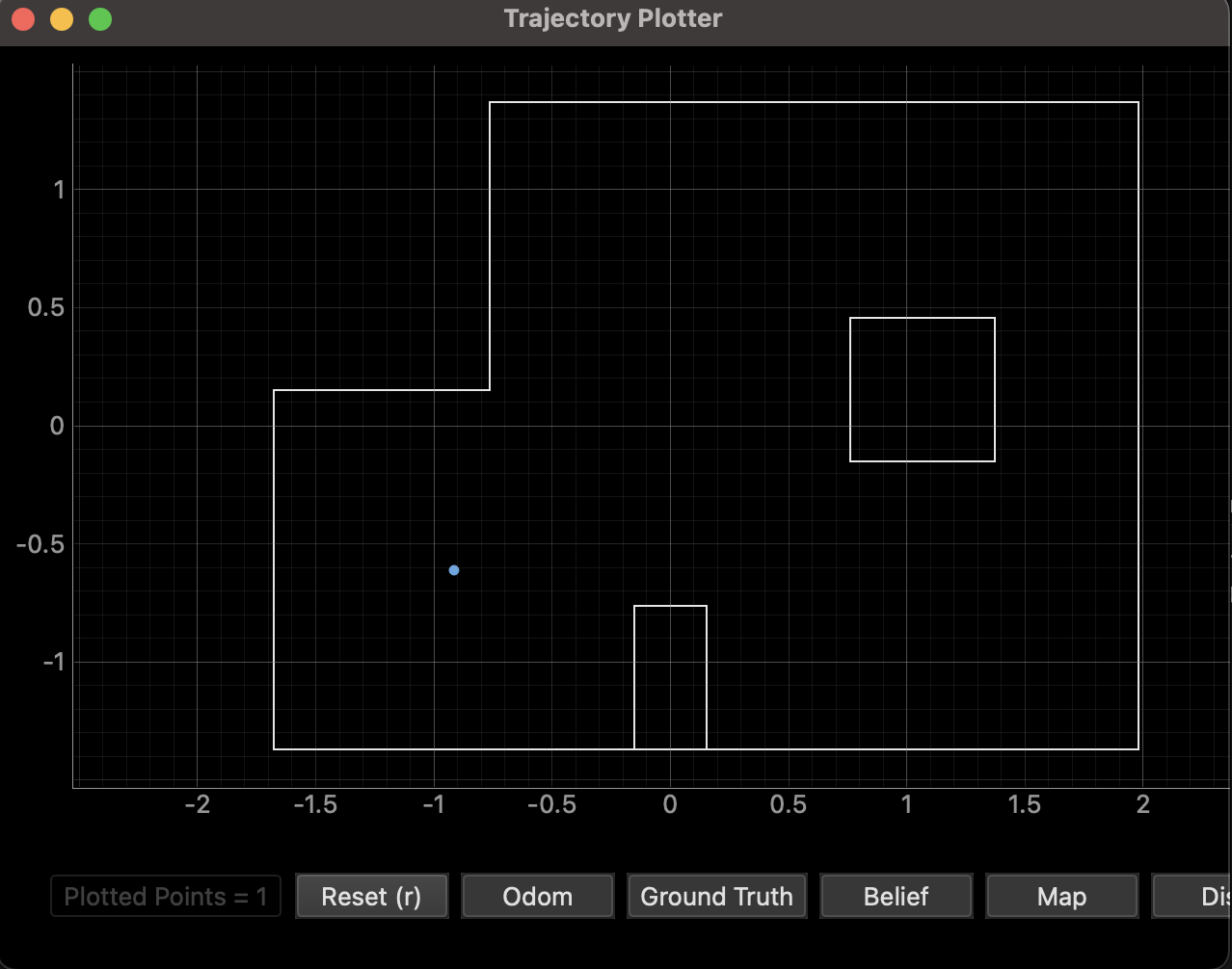
(-3, -2) / (-0.91m, -0.61m):

The localization was excellent. The peak belief in the final grid aligned almost perfectly with the ground truth marker. I had to record a video showing the toggling of the belief and ground truth to show that they overlay each other.

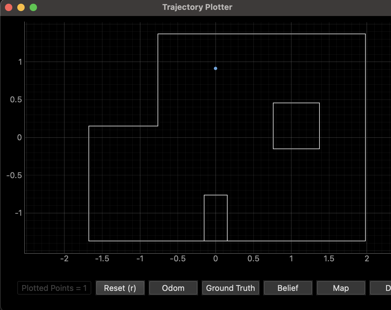
(0, 3) / (0m, 0.91m):

Similar to the previous pose, the localization was very accurate. The belief grid showed a strong peak matching the ground truth position and orientation.

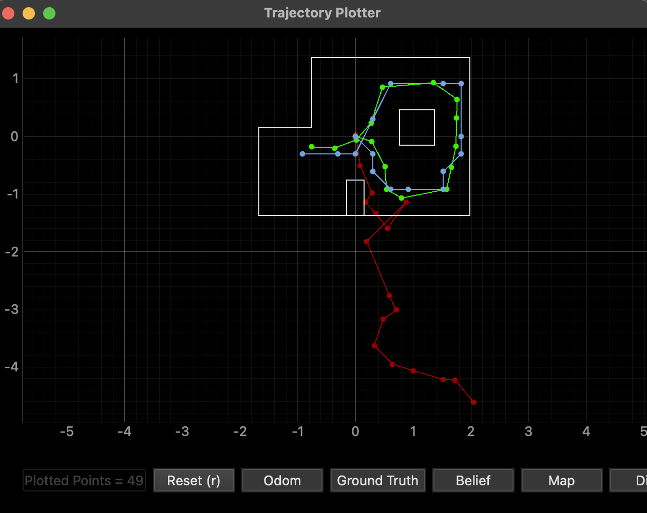
(5, -3) / (1.52m, -0.91m)

The localization was good. The belief peak was very close to the ground truth. (As noted, data wasn't saved initially, so plots were generated separately, showing good alignment).

Belief Grid at (5, -3)

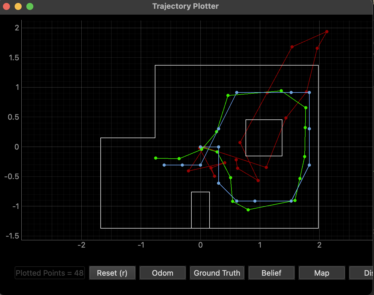
Ground Truth at (5, -3)

(5, 3) / (1.52m, 0.91m):

At this location, there was a noticeable discrepancy. While the belief grid converged to a single peak, this peak was offset from the ground truth marker by almost 1 tile in y.

Belief Grid vs Ground Truth at (5, 3)

Although I tried to place the robot accurately, a small error in the starting position or, more likely, the initial orientation (even 5-10 degrees off 0) could significantly affect which grid cell receives the highest likelihood, especially if the true pose is near a cell boundary. A few erroneous ToF readings during the scan at that specific location due to the open nature of the location could skew the likelihood calculation making the belief offset from the ground truth.

Conclusion

This lab successfully demonstrated the application of the Bayes filter's update step for localizing a real robot within a known map, starting from a uniform prior. By using a single 360-degree sensor scan, the robot could often determine its position and orientation with good accuracy, despite the absence of a motion model prediction step. The process highlighted the differences between simulation and reality. While the core algorithm worked, factors like precise initial robot placement, potential map inaccuracies from Lab 9, and real-world sensor noise demonstrably affected the final localization quality, leading to near-perfect results in some locations and minor offsets in others. Overall, the experiment validates the power of probabilistic sensor fusion for localization. Even with noisy sensors and imperfect maps, correlating sensor readings with the environment model via the Bayes update step provides a robust way to estimate the robot's pose, far surpassing what could be achieved with odometry alone on this hardware.

Credits

[1] Stephan Wagner