Mapping

Author: Akinfolami Akin-Alamu

The purpose of this lab was to generate a 2D map of a known environment (in the lab) by taking Time-of-Flight (ToF) sensor readings from multiple known locations. This map will serve as the basis for future localization and navigation tasks.

Setup

For this lab, I needed a reliable way to rotate the robot and take sensor readings at consistent angular intervals. The lab instructions offered three approaches: open-loop, orientation PID control, and angular speed PID control. Given my success with the orientation PID controller using the IMU's DMP in Lab 6 and Lab 8, and the instructions noting that stationary readings improve ToF accuracy, I decided to pursue the Orientation Control method (Option 2). This approach promised better accuracy than open-loop without requiring the implementation of a new angular speed controller.

The plan was to reuse the existing orientation PID controller and DMP setup. I would program the robot to turn to specific angular setpoints, stop, take a ToF reading, and repeat this process for a full 360-degree rotation. This "step-and-scan" method seemed like a good balance between accuracy and implementation complexity. Fortunately, most of the required code infrastructure (DMP initialization, PID function, BLE communication) was already in place from previous labs.

Lab Tasks

Control Implementation: Step-and-Scan

The core of the mapping process was implemented in my Arduino loop() function. Instead of continuous rotation, I opted for a sequence of discrete turns. When the START_PID command is received (is_pid_running becomes true), the robot performs a series of turns.

1. It records the starting yaw angle (start_yaw).
2. It iterates 15 times (for step 0 to 14). In each iteration:
   • A new pid_target angle is calculated: start_yaw + (step * 25). This creates target increments of 25 degrees.
   • A do-while loop engages the pid_control() function to drive the motors (turn_around()) until the current yaw (yaw_gy) is within a 3-degree tolerance of the pid_target.
   • The robot stops (stop()).
   • A ToF reading is taken using distance_sensor_1.
   • The timestamp, current yaw (imu_vals), final PWM (pwm_vals), and ToF distance (tof_vals) are logged.
3. After the loop, a final turn to start_yaw + 360 degrees is performed to ensure a reading close to the starting point, completing the full circle.
4. The process stops (is_pid_running = false).

A crucial addition from previous labs was the wrap()_angle function. Since the robot rotates more than 180 degrees, the raw yaw_gy output from atan2 (which is between -180 and +180) needs to be unwrapped to represent continuous rotation (e.g., going from 170 to -170 should become 170 to 190). This function handles the wrap-around logic, ensuring the PID controller targets and tracks angles correctly beyond +/-180 degrees.

// Inside loop() when is_pid_running is true:
      float start_yaw = yaw_gy;
      for (int step = 0; step <= 14; step++) { // 15 steps for 0 to 350 degrees
        pid_target = start_yaw + (step * 25); // Increment target by 25 deg

        // Turn to target angle
        do {
          record_dmp_data(); // Updates yaw_gy using wrap()_angle()
          pwm = pid_control(yaw_gy);

          // Scale PWM and drive motors using turn_around()
          int scaled_pwm = map(abs(pwm), 0, 255, 70, 255);
          if (pwm > 0) {
            turn_around(1, scaled_pwm, 1.25);
          } else if (pwm < 0) {
            turn_around(0, scaled_pwm, 1.25);
          }

        } while (abs(yaw_gy - pid_target) >= 3.0); // Turn until within 3 degrees
        stop();

        // Take ToF Reading
        distance_sensor_1.startRanging();
        while (!distance_sensor_1.checkForDataReady()) { delay(1); }
        int distance = distance_sensor_1.getDistance();
        distance_sensor_1.clearInterrupt();
        distance_sensor_1.stopRanging();

        // Log Data
        if (curr_idx < MAX_DATA_SIZE) {
          times[curr_idx] = (float)millis();
          pwm_vals[curr_idx] = pwm; // Log last pwm command
          imu_vals[curr_idx] = yaw_gy; // Log actual angle achieved
          tof_vals[curr_idx] = distance;
          curr_idx++;
        }
      }
      // Perform final turn to 360 degrees from start
      pid_target = start_yaw + 360;
      do {
        // ...turn logic similar to above...
      } while (abs(yaw_gy - pid_target) >= 3.0);
      stop();
      // ...take final ToF Reading and Log Data ...

      is_pid_running = false;
      stop();

Data Acquisition

I placed the robot at the four specified locations in the lab: (-3,-2), (0,3), (5,3), and (5,-3). At each location, I tried to align the robot facing roughly the same direction (positive X-axis of the room frame) before starting the scan using the START_PID BLE command. After each 360-degree scan completed, I used the SEND_PID_DATA command to transfer the logged time|imu|pwm|tof data back to my laptop via Bluetooth, saving each scan to a separate CSV file named according to the robot's position (e.g., robot_data_..._(-3,-2).csv). This turned out to be very handy for post-processing the data later.

Here's a short video showing the robot performing the step-and-scan routine: Despite my best efforts, note how there is some non-negligible drift from the starting position. It was difficult to rotate perfectly about that axis, so the drift was accounted for in the post-processing step.

Sanity Check: Polar Plots

Before merging the data, I generated polar plots for each individual scan in Python. This helped visualize the shape of the room from each viewpoint and check for any obvious errors or inconsistencies in the readings. The angles used were the actual recorded IMU angles (imu_vals). The method to generate the polar plots is given below. The same method was re-used in later steps

// file_names is a list of filenames
for idx, (filename, ax) in enumerate(zip(file_names, axes_polar)):
    with open(filename, newline='') as csvfile:
        reader = csv.reader(csvfile)
        next(reader)  # Skip header
        results = [[float(x) for x in row] for row in reader]

    imu_angles_deg = np.array([row[1] for row in results])
    tof_readings = np.array([row[3] for row in results])
    imu_angles_rad = np.radians(imu_angles_deg)

    ax.plot(imu_angles_rad, tof_readings, 'o-')
    ax.set_rmax(max(tof_readings) * 1.1)
    ax.set_rticks(np.linspace(0, ax.get_rmax(), 5))
    ax.set_rlabel_position(-22.5)
    ax.grid(True)

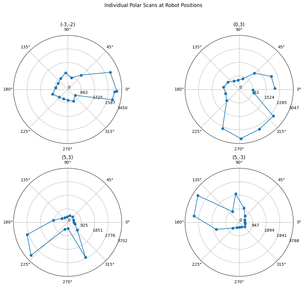Individual Polar Scans

The plots generally matched expectations (also comparing with friends), showing shorter distances towards nearby walls and longer distances in open areas. The ~25-degree increments were visible.

Transformation to World Frame

To merge the scans, each ToF reading needed to be converted from the sensor's frame to the global room frame (world frame). I referred to the Transformation Matrices provided in lecture for this.

The transformation chain is: P_i = T_R * T_TOF * P_TOF

Where:

• P_TOF = [r, 0, 1]^T is the point detected by the TOF sensor in the sensor frame (distance r along its x-axis).
• T_TOF transforms from sensor to body frame. Since the sensor is mounted in front of the car at approximately 70mm (l = 0.070m) along the robot's x-axis with no rotation: T_TOF = [[1, 0, 0.070], [0, 1, 0], [0, 0, 1]]
• T_R transforms from body frame to world frame. For a robot at (x, y) with yaw θ (from IMU): T_R = [[cosθ, -sinθ, x], [sinθ, cosθ, y], [0, 0, 1]]

Combining these, a point P_TOF transforms to P_i which ultimately simplifies to: P_i = [[(l+r)cosθ + x], [(l+r)sinθ + y], [1]] after multiplying it out.

This means the world coordinates (x_world, y_world) are: x_world = x + (l + r) * cos(θ) y_world = y + (l + r) * sin(θ)

Where l = 70mm, r is the ToF reading (in mm), (x, y) is the robot's known position (in mm), and θ is the corresponding IMU yaw angle (in radians).

Merging Readings

I created a python function to apply this transformation to all points from the four CSV files. Additionally, I generated a scatter plot of the resulting world frame positions. Plotting the initial data revealed some misalignments. As I mentioned earlier, the robot was not perfectly aligned with the starting position, so the raw data was a little tilted compared to how it should have been. I adjusted for this using an offset which I applied to all the angles. I tuned this angle experimentally. My function to apply this transformation and the offset is given below. Note I also converted the coordinates to meters for easier plotting.

  l_sensor_mm = 70.0
  imu_deg = []
  tof_mm = []
  with open(file_name, newline="") as f:
      reader = csv.reader(f)
      next(reader)
      for t, imu, pwm, tof in reader:
          imu_deg.append(float(imu)+offset)
          tof_mm.append(float(tof))
  imu_rad = np.radians(imu_deg)

  global_x = []
  global_y = []
  for θ, r in zip(imu_rad, tof_mm):
      d = r + l_sensor_mm
      global_x.append((d * math.cos(θ)) / 1000.0)
      global_y.append((d * math.sin(θ)) / 1000.0)

The following plots plots before show a before and after comparison applying offsets to the data.

(-3,-2) Before vs After

(-3,-2) Transformation to world frame (Before Offset)(-3,-2) Transformation to world frame (After offset)

(0,3) Before vs After

(0,3) Transformation to world frame (Before Offset)(0,3) Transformation to world frame (After offset)

(5,3) Before vs After

(5,3) Transformation to world frame (Before Offset)(5,3) Transformation to world frame (After offset)

(5,-3) Before vs After

(5,-3) Transformation to world frame (Before Offset)(5,-3) Transformation to world frame (After offset)

After Applying these offsets I was able to merge the scatter plots using a similar method as before. I start by computing the transformations and saving it in an array. I can then plot this array one by one on the same plot. In the code below, the method to compute the transformations (from above) has been moved to a separate function called global_points.

for fname, c, offset in zip(file_names, colors, offsets):
    xs, ys, lbl = global_points(fname, offset)
    plt.scatter(xs, ys, s=8, color=c, label=lbl)

And here is the final merged map:

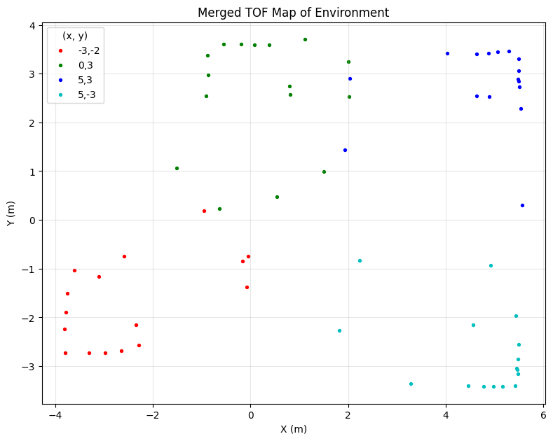Offset-Corrected Merged Scatter Plot

Creating the Line-Based Map

With the corrected scatter plot showing the room's structure, the final step was to manually interpret the points and draw straight lines representing the walls and major obstacles. I added lines based on the visual clusters of points.

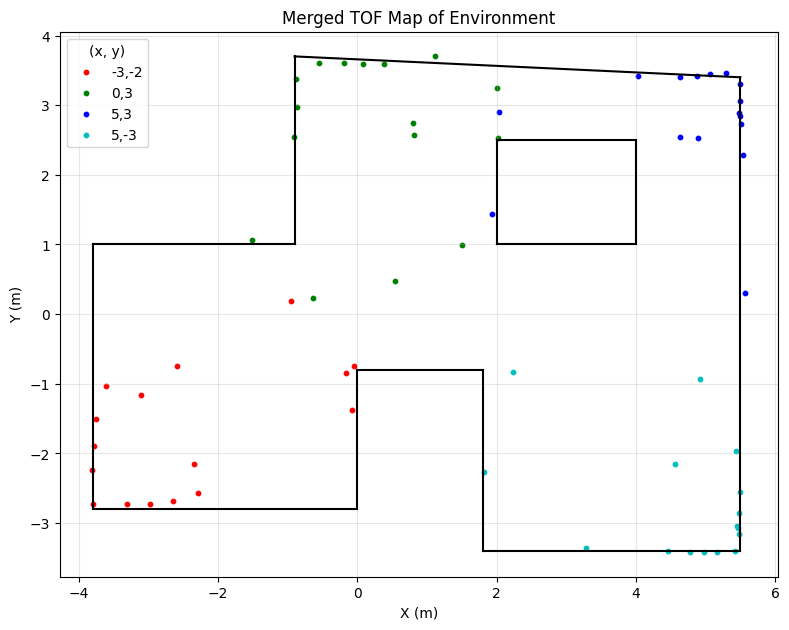Final Line-Based Map

The lines were added using the following x,y pairs of coordinates. These will serve as x_start, y_start to be used in the simulation for next lab.

lines= [
    ((1.8, -3.4), (5.5, -3.4)),   
    ((5.5, -3.4), (5.5,  3.4)),    
    ((5.5,  3.4), (-0.9,  3.7)),    
    ((-0.9,  3.7), (-0.9,  1.0)),  
    ((-3.8,  1.0), (-0.9,  1.0)),   
    ((0.0,  -0.8), (0.0, -2.8)),  
    ((-3.8, -2.8), (-0.0, -2.8)),  
    ((-3.8, -2.8), (-3.8, 1.0)),  
    ((0.0, -0.8), (1.8, -0.8)),  
    ((1.8, -0.8), (1.8, -3.4)),  
    # ── square interior obstacle ──
    ((2.0,  1.0), (4.0,  1.0)),   
    ((4.0,  1.0), (4.0,  2.5)),  
    ((4.0,  2.5), (2.0,  2.5)),      
    ((2.0,  2.5), (2.0,  1.0)), 
]

This line-based map provided a simplified representation of the environment suitable for use in simulation or path planning algorithms in later labs. Although, the data was not perfect, it was a fairly decent approximation of the environment given in the lab.

Conclusion

Reusing the PID and DMP code from previous labs made this lab very efficient. The main challenge was the initial misalignment between scans, highlighting the sensitivity to the robot's starting orientation and potential minor inconsistencies in IMU readings across different runs. Applying manual angular offsets during post-processing was enough but still slightly off to create a coherent final map.