Path Planning and Execution

Author: Akinfolami Akin-Alamu

The purpose of this lab was to integrate all previously developed systems (mapping, localization, and control) to enable the robot to navigate a series of waypoints within the known environment. This lab was intentionally open-ended, encouraging us to tailor a solution best suited to our robot's capabilities.

Design

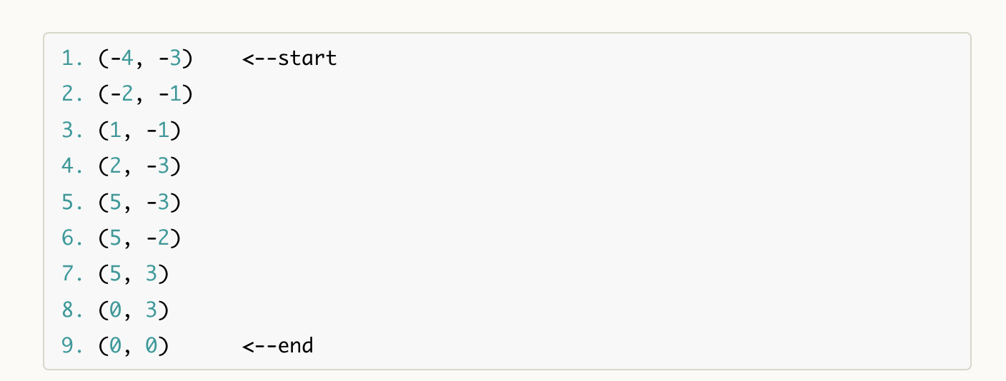
The grand vision was to create a semi-autonomous navigation system. My initial plan, building upon the successful localization from Lab 11, was to implement a state machine that would:

Localize: Perform a 360-degree scan and run the Bayes filter update step (as in Lab 11) to determine the robot's current pose (position and orientation).
Calculate Heading: Given the current localized pose and the next target waypoint, calculate the required change in heading (angle to turn).
Turn: Use the IMU-based orientation PID controller (from Lab 6, 9, 11) to turn the robot to face the next waypoint.
Drive: Drive forward a calculated distance towards the waypoint.
Repeat for all waypoints.

Since I planned to rely on accurate localization and open space between waypoints, I didn't need to bother about complex obstacle avoidance. I also decided to skip complex graph search algorithms like A*. Given the relatively simple environment and predefined waypoints, a direct "go-to-next-waypoint" approach seemed sufficient. Additionally, my approach relied heavily on already developed code from previous labs which was great to connect everything together. For example, orientation PID control using the IMU's DMP was a clear choice, as it had proven reliable for more than 3 labs. Driving in a straight line was a bit more tricky. My thought was to drive open-loop for a calculated duration. I was hesitant to use ToF-based distance control for forward movement, as the sensor might be pointing at an odd angle during a forward movement or towards an area not ideal for reliable distance to the target, especially if the target was far (or even constantly changing).

As a side note, the system would be primarily driven from the Jupyter Notebook. The notebook would manage the state machine, because we need to compute the belief at each waypoint and send commands to the Arduino to localize, turn to angle, drive for duration.

Code

To support this state machine, I extended the Arduino code from Lab 11 with new BLE commands and refined existing ones:

LOCALIZE Command (New): This command triggers the 18-step, 20-degree-increment scan routine developed in Lab 11. Upon completion, the Arduino collects ToF readings and IMU yaw values. It then sends a "DONE" message back via BLE to signal the Python script that the scan data is ready for transmission.

// In handle_command()
case LOCALIZE: {
    localize(); // Executes the 18-step scan
    // Reset PID states for next potential PID action
    accumulated_error = 0.0;
    last_pid_time = millis();
    curr_idx = 0; // Reset data buffer index for next SEND_PID_DATA
    break;
}

SET_SETPOINT Command (Modified): This command was adapted to accept a relative target angle. The Jupyter Notebook calculates the absolute angle needed to face the next waypoint. It then computes the difference between this absolute target and the robot's current localized orientation. This difference (the angle to turn) is sent to the Arduino. The Arduino adds this relative angle to its current yaw_gy to set the new pid_target. Below is the code from the Jupyter Notebook that calculates the angle to turn.

def angle_to_turn(src, dst):
    dx = dst[0] - src[0]
    dy = dst[1] - src[1]
    return math.atan2(dy, dx)

DRIVE Command (New): This command was intended for open-loop straight driving. It would take a duration (in milliseconds) as a parameter and drive the robot forward at a fixed PWM for that time.

// In handle_command()
case DRIVE: {
    int time_to_drive;
    success = robot_cmd.get_next_value(time_to_drive);
    if (!success) { return; }
    Serial.print("Driving straight for ms: ");
    drive_in_a_straight_line(1, 200, 1.25);
    delay(time_to_drive);
    stop();
    break;
}

The Reality: A Necessary Pivot

We (me and Tony) meticulously implemented the Arduino changes and the Python logic. The individual components—localization via LOCALIZE, PID turning via SET_SETPOINT, and timed driving via DRIVE—all seemed to function correctly in isolation when tested individually.

However, when we attempted to run the full waypoint navigation sequence, we encountered a deeply frustrating issue: the robot often wouldn't move consistently, or at all, especially during the crucial PID-controlled turns. Despite the motors audibly whirring and the PID controller outputting non-zero PWM values (verified via serial prints and the pwm_vals logging from previous labs), the robot would frequently get stuck or only jitter slightly.

This was incredibly disheartening. We suspected several culprits:

Battery Level: Even with freshly charged batteries, the issue persisted.
Friction: The lab floor, while generally smooth, might have had "sticky" spots for our particular wheels/chassis.
Motor/Driver Issues: Perhaps the motor drivers weren't delivering enough current, or the motors themselves were underpowered for precise, low-speed maneuvers from a standstill, especially for turning on the spot (which requires overcoming significant static friction for two wheels to slip).

With the deadline rapidly approaching, and after many hours of troubleshooting the motion issues, we had to make a pragmatic decision to pivot. The fully integrated, closed-loop navigation dream was, for our specific robot at this moment, out of reach.

The Pivot: Open-Loop Navigation

To demonstrate some form of waypoint navigation, we fell back to a purely open-loop strategy for the entire path. This meant abandoning the per-waypoint localization and PID-controlled turns. Instead, we hardcoded a sequence of timed forward drives and turns into a new Arduino function, open_loop_drive(). This function was then triggered by the DRIVE command from Python, effectively making the DRIVE command execute the entire pre-programmed path.

void open_loop_drive() {
  Serial.println("Driving in a straight line");
  // from (-4,3) to (-2, -1)
  drive_in_a_straight_line(1, 100, 1.25);
  delay(1000);
  stop();
  delay(1000);
  Serial.println("Stopped after first straight line");

  turn_right(100);
  delay(1000);
  stop();
  delay(1000);

  Serial.println("Stopped after first right turn");

  drive_in_a_straight_line(1, 100, 1.25);
  delay(1000);
  stop();
  delay(1000);

  Serial.println("Stopped after second straight line");

  turn_left(100);
  delay(500);
  stop();
  delay(1000);

  Serial.println("Stopped after second right turn");

  drive_in_a_straight_line(1, 100, 1.25);
  delay(800);
  stop();
  delay(1000);
  Serial.println("Stopped after third straight line");

  turn_left(100);
  delay(500);
  stop();
  delay(1000);

  Serial.println("Stopped after first left turn");

  drive_in_a_straight_line(1, 100, 1.25);
  delay(1000);
  stop();
  delay(1000);
  Serial.println("Stopped after fourth straight line");

  turn_left(100);
  delay(500);
  stop();
  delay(1000);
  Serial.println("Stopped after second left turn");

  drive_in_a_straight_line(1, 100, 1.25);
  delay(1000);
  stop();
  delay(1000);
  Serial.println("Stopped after fifth straight line");

  turn_left(100);
  delay(500);
  stop();
  delay(1000);
  Serial.println("Stopped after third left turn");

  drive_in_a_straight_line(1, 100, 1.25);
  delay(1000);
  stop();
  delay(1000);
  Serial.println("Stopped after sixth straight line");

  drive_in_a_straight_line(1, 100, 1.25);
  delay(1000);
  stop();
  delay(1000);

  Serial.println("Stopped after final straight line");
  Serial.println("Done driving");
}

The DRIVE case in handle_command() was simplified to just call this:

    case DRIVE: {
    open_loop_drive();
    break;
}

The PWM values and delay durations in open_loop_drive() were determined through painstaking trial and error, attempting to make the robot roughly trace the waypoint path.

Results

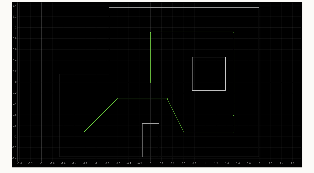
The open-loop approach, while a significant departure from the initial plan, did allow the robot to physically move through the environment in a sequence that approximated the waypoint path.

The open-loop approach achieved moderate accuracy. The robot slightly deviated from the intended path due to the lack of feedback and localization, but maintained a general trajectory toward the target area. The tuned PWM values and delay timings enabled basic execution of turns and straight segments. While this demonstrated the feasibility of timed maneuvers for simple navigation, a closed-loop system would have provided better precision and reliability.

Conclusion

Lab 12 was an ambitious undertaking, aiming to tie together everything we'd learned. My initial design for a closed-loop system with intermittent localization and PID-controlled turns was, I believe, sound in principle. Despite not achieving the fully closed-loop navigation, this lab has been an incredible learning experience. Across all labs, from soldering components and debugging low-level hardware, to implementing sophisticated algorithms like PID control, Kalman Filters, and Bayes Filters, the journey has been immensely rewarding. The hands-on nature of these labs provided insights that lectures alone cannot.

The challenges in this final lab serve as motivation rather than discouragement. They highlight areas for future improvement. Most importantly, better mechanical design (my robot couldn't flip for this reason) for lower friction, or more advanced control and planning strategies. I've thoroughly enjoyed Fast Robots and look forward to applying these skills and tackling more robotics projects in the future.