Stunts

Author: Akinfolami Akin-Alamu

The purpose of this lab was to combine the functionalities developed in previous labs – specifically the Kalman Filter for distance estimation (Lab 7) and the IMU-based orientation PID control (Lab 6) to execute a dynamic stunt. The goal for my chosen stunt, Task B: Drift, was to make the car drive forward quickly towards a wall, initiate a 180-degree turn upon reaching a specific distance (3ft / 914mm), and briefly drive back.

Planning the Stunt

This lab felt like the culmination of the previous weeks' work. The core components needed were already implemented: the Kalman Filter from Lab 7 for robust distance estimation even with potentially intermittent ToF readings, and the orientation PID controller using the IMU's DMP from Lab 6 for controlling the car's yaw angle.

The main task was integrating these systems into a cohesive state machine that could handle the different phases of the drift stunt:

Fast forward approach using KF/ToF distance.
Triggering the turn at the correct distance.
Executing a rapid 180-degree turn using orientation PID.
A brief reverse drive after the turn.

Fortunately, the infrastructure from Labs 6 and 7 was largely reusable. I kept the DMP configuration for the IMU identical to Lab 6 to get reliable yaw readings (yaw_gy) and the Kalman Filter setup (matrices A, B, C, Ad, Bd, noise parameters sig_u, sig_z) exactly as tuned in Lab 7.

Lab Tasks: Implementing the Drift

The core logic for the drift was implemented within a new state machine managed by the is_drift_running flag and a sub-state flag drift_flag. A new command START_PID (which I probably should have renamed START_DRIFT from last lab) triggers the start_drift() function.

The start_drift() function initializes the necessary components:

Gets an initial ToF reading to seed the Kalman Filter state (mu).
Resets the KF covariance matrix sigma.
Sets is_drift_running to true and drift_flag to false (indicating the initial forward drive phase).
Resets data logging variables and PID controller states (accumulated_error, prev_error).
Starts the ToF sensor ranging.

void start_drift() {
  Serial.println("Starting drift routine...");
  distance_sensor_1.startRanging();
  // Wait for the first valid distance reading
  while (!distance_sensor_1.checkForDataReady()) {
    delay(1);
  }
  int current_distance = distance_sensor_1.getDistance();
  distance_sensor_1.clearInterrupt();
  distance_sensor_1.stopRanging(); // Stop continuous ranging briefly

  // Initialize Kalman filter state with the first reading
  mu = {(float)current_distance, 0.0}; // Assume initial velocity is 0
  sigma = {sigma_3 * sigma_3, 0, 0,
           100}; // Reset covariance (position variance based on sensor,
                 // velocity variance high)

  is_drift_running = true;
  drift_flag = false; // Start in the forward driving phase
  start_time_drift = millis();
  curr_idx = 0;             // Reset data logging index
  accumulated_error = 0.0;  // Reset PID integral term
  prev_error = 0.0;         // Reset PID derivative term
  last_pid_time = millis(); // Initialize PID timer

  distance_sensor_1.startRanging(); // Restart continuous ranging
}

The main logic resides in the drift() function, called repeatedly from the loop() when is_drift_running is true.

Phase 1: Forward Drive

When drift_flag is false, the car drives forward at a constant drive_forward_speed (set to 255 for maximum speed). I mostly used the same code from Lab 7 to get the ToF readings and update the Kalman Filter state. I always make sure to run the predict step, However, if a new ToF reading is available the KF update step (kf_update()) is called using the raw distance.

int raw_distance = -1;
  if (distance_sensor_1.checkForDataReady()) {
    raw_distance = distance_sensor_1.getDistance();
    distance_sensor_1.clearInterrupt();
    distance_sensor_1.stopRanging(); // Necessary cycle for VL53L1X
    distance_sensor_1.startRanging();
    kf_update(mu_p, sigma_p, mu, sigma, raw_distance); // Update step
  }
  // Use raw distance if available, otherwise use KF estimate
  int effective_distance = (raw_distance != -1) ? raw_distance : (int)mu(0, 0);

The car continues forward until effective_distance drops below the drift_point (914mm).

if (!drift_flag) { // Phase 1: Driving forward
    if (effective_distance > drift_point) {
      drive_in_a_straight_line(1, drive_forward_speed, 1.25); // Drive forward (direction 1)
      // ... data logging ...
    } else {
      drift_flag = true; // Reached drift point, switch to turning phase
      reverse_start_time = millis();
    }
  } else { // Phase 2: Turning and Reversing
    // ... see below ...
  }

Phase 2: Turning and Reversing

Once drift_flag becomes true, the car switches to the turning phase. Here, the orientation PID controller from Lab 6 takes over. The pid_control(yaw_gy) function calculates the necessary PWM output based on the difference between the current yaw (yaw_gy from DMP) and the pid_target (180 degrees).

The calculated PWM determines the turning direction and speed using a turn_around() (same from lab 6) function, which implements differential drive. I added a scaling step (map()) to ensure the motors overcome static friction and the deadband, using a minimum PWM of 150 when turning.

// In drift() function, phase 2:
if (abs(pid_target - yaw_gy) > 5) { // Turn until close to target (5 degree tolerance)
    pwm = pid_control(yaw_gy);
    // ... data logging ...

    if (abs(pwm) > 0) {
      int scaled_pwm;
      if (pwm > 0) { // Turn one way
        scaled_pwm = map(pwm, 0, 255, 150, 255);
        turn_around(1, scaled_pwm, 1.25); // Assumes direction 1 is correct for positive PWM error
      } else { // Turn the other way
        scaled_pwm = map(abs(pwm), 0, 255, 150, 255);
        turn_around(0, scaled_pwm, 1.25); // Assumes direction 0 is correct for negative PWM error
      }
    } else {
      stop();
    }
} else { // Phase 3: Target angle reached, drive back briefly
    drive_in_a_straight_line(0, drive_back_speed, 1.25); // Drive backward (direction 0)
    // ... data logging ...
    if (millis() - reverse_start_time > REVERSE_DURATION) { // Drive back for fixed duration
      stop();
      is_drift_running = false; // End of stunt
      distance_sensor_1.stopRanging();
      // distance_sensor_2.stopRanging(); // Not used in drift logic
    }
}

Once the yaw angle is within 5 degrees of the 180-degree target, the car stops turning and drives back to the start point at drive_back_speed for a fixed REVERSE_DURATION (1400ms). After this, the motors stop, is_drift_running is set to false, and the stunt sequence is complete. Below are videos demonstrating successful drift runs:

And here is a plot showing the sensor data, KF estimate, yaw angle, and PWM output. My Kalman Filter didn't turn out to be reliable enough. But we can see the change in angle for the drift.

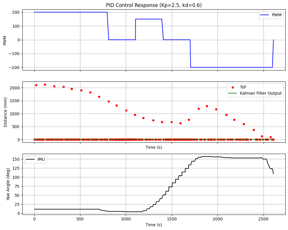Drift Stunt Data Plot

Conclusion

This lab was a fantastic way to integrate multiple complex systems developed previously. Successfully combining the Kalman Filter for state estimation under speed and the orientation PID for dynamic control felt like a significant achievement. The state machine approach worked well to manage the distinct phases of the stunt. Although, I was frustrated because I couldn't get my car to flip over, I was comfortable with the success of the drift.

[1] Insights from Lab 6 on DMP configuration [https://fast.synthghost.com/lab-6-orientation-pid-control/](Stephan Wagner (2024)) and Lab 7 on KF initialization (Stephan Wagner (2024)) were again very helpful as starting points.