Time of Flight Sensors
The purpose of this lab was to setup the VL53L1X Time-of-Flight(ToF) sensor. It involved analyzing the accuracy and reliability of both sensors, as well as making them work in parallel.
Prelab
The VL53L1X ToF datasheet can communicate over I2C as documented in the datasheet. The default I2C device address is 0x52. However, the I2C is only 7 or 10 bit adressible. In the 7-bit addressing mode (which is what we will be using), the LSB of the address is used to select the read/write mode of the device. Hence, the board will use 0x29 (upper 7 bits) as the I2C address for the VL53L1X.
Using Both ToF Sensors
Since both sensors are VL53L1X, they share the same I2C address, However, we want to communicate with them independently. To do this, we need to programmatically change the I2C address of one
of the sensors during the setup phase. This done by first taking the XSHUT pin of the other sensor low which puts the sensor in shutdown mode, effectively disconnected from the I2C bus. This way, the other sensor will not be affected by the I2C address change. Then, we configure the new address,
and finally raise the XSHUT pin of the other sensor to high.
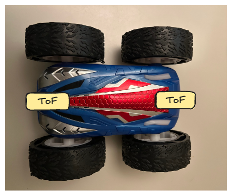
Placement of ToF Sensors
I decided to place one ToF sensor in the front of the robot and the other in the back. This way, the sensors will be able to see obstacles in front of it. The sensors will also be able to see the robot in the back, which will help navigate quickly if
the robot is approaching an obstacle from either side.
 ToF Setup
Wiring
I wired the the VL53L1X sensors using the following sketch from Wenyi Fu
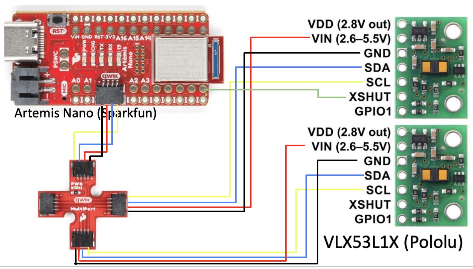
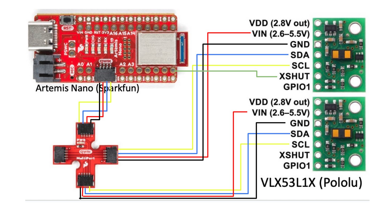 ToF Wiring
Lab Tasks
Soldering the battery wires to JST jumper wires
I cut the original wire on the 650mAh battery (one by one, of course) and then soldered the wires to the JST jumper wires, which
could then be cnnected to the Artemis to power it!
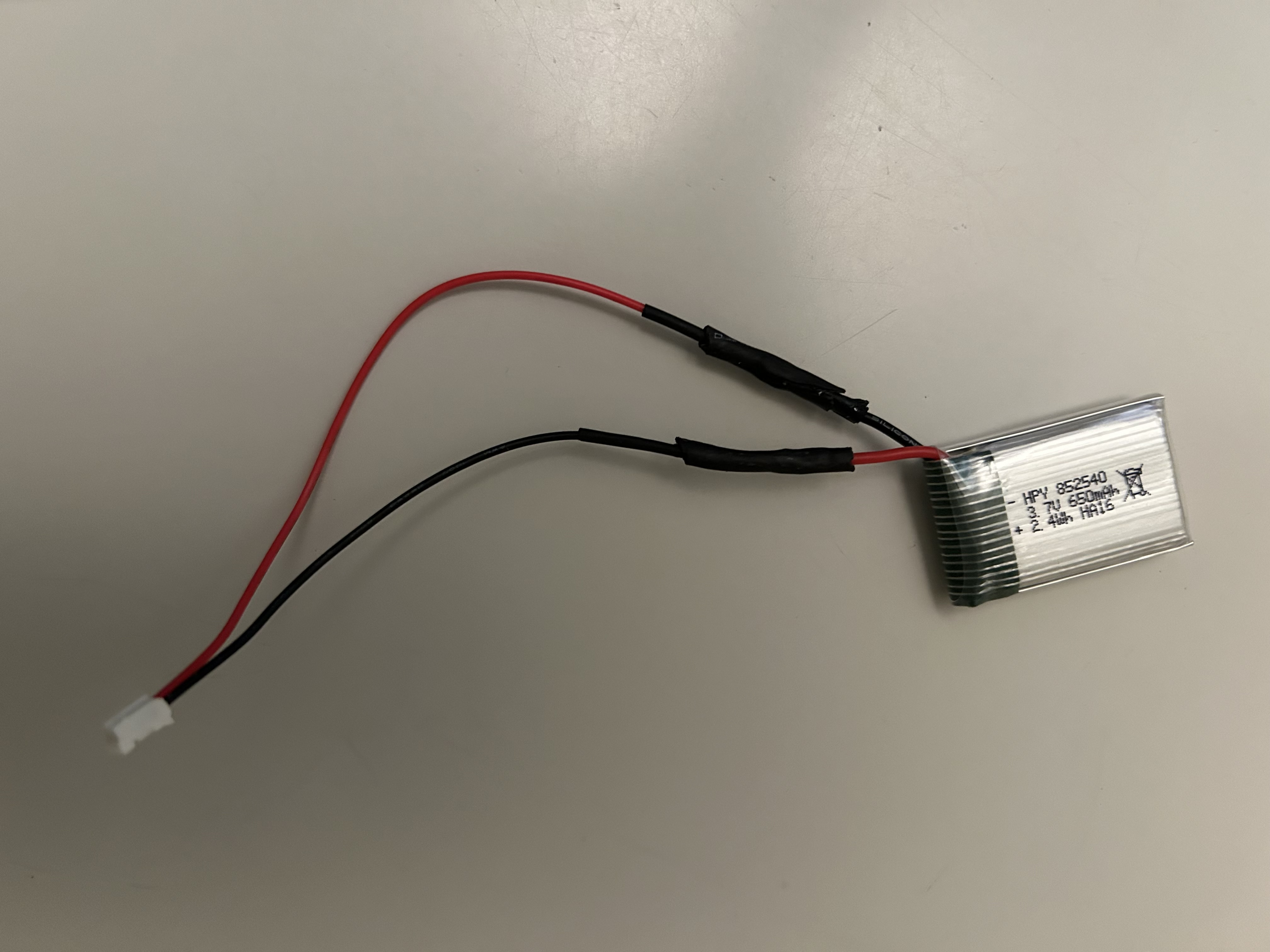 650mAh Battery
Sending BLE messages using battery powered Artemis
And we can see that the board is powered by the battery!
Picture of ToF sensor connected to your QWIIC breakout board
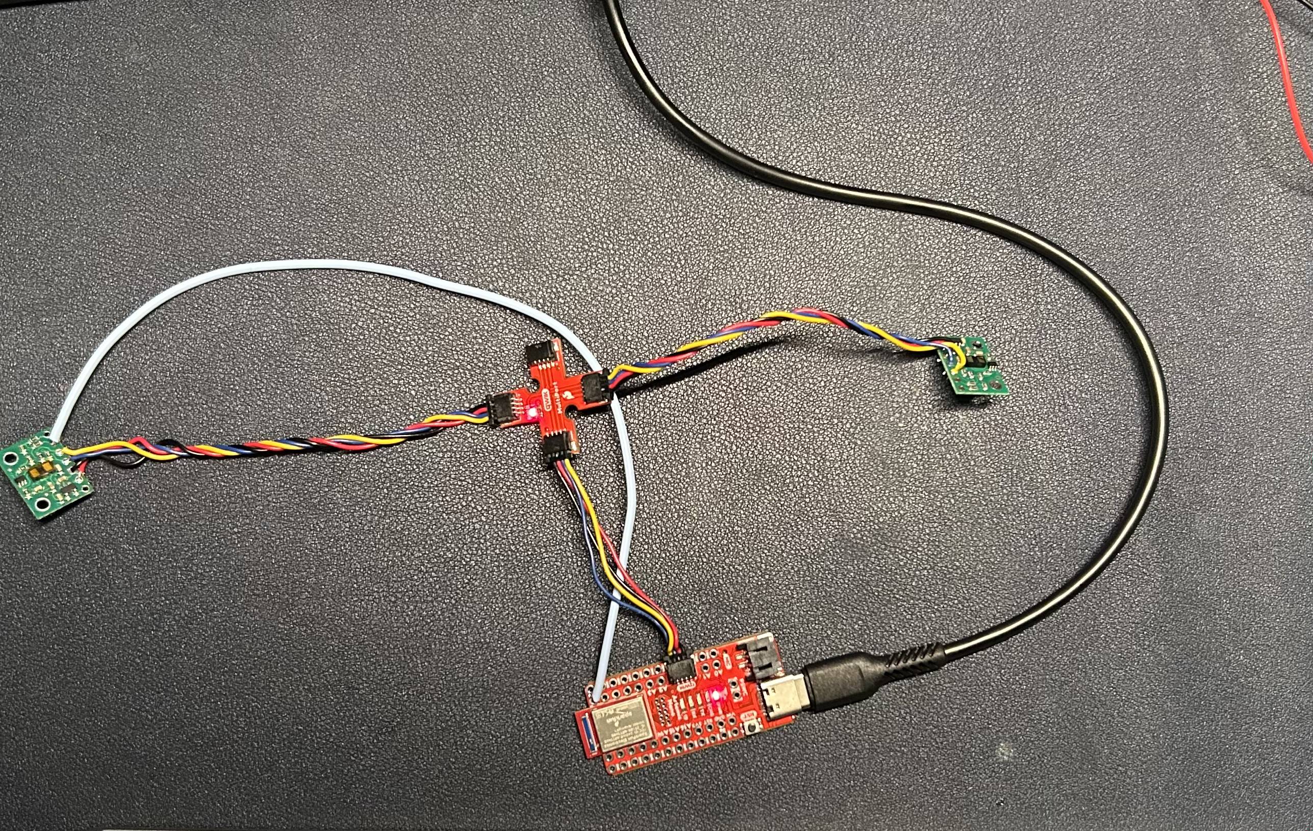
The ToF sensors were connected to the QWIIC breakout board and the Artemis as in the image below.
Screenshot of Artemis scanning for I2C device
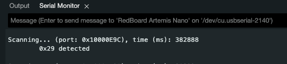
The Artemis was scanning for the I2C device of the ToF sensors. As discussed earlier, the effective address of the VL53L1X works out to 0x29.
The board was able to find the ToF sensor and print out the following message to the serial monitor.
Discussion of sensor data with chosen mode
The two (short and long) different distance modes have their pros and cons. 20ms is the minimum timing budget and can only be used in short distance mode. However,
short distance mode only has a range of (0.05-1.3m). On the other hand, 140ms is the timing budget which can allow for a maximum distance of 4m which can only
be reached in long distance mode. Overall, 33ms is the minimum timing budget that can work for all modes, and a higher timing budget means improved reliability
on the sensors. Considering we are developing a fast robot, we want the sensor to return a distance to us fairly quickly. Additonally, it makes more sense to track obstacles that are closer
to the robot car. I think a short distance mode which gives reasonable range and a timing budget of 33ms for improved reliability
would be a good choice for a distance mode.
Testing the short distance mode
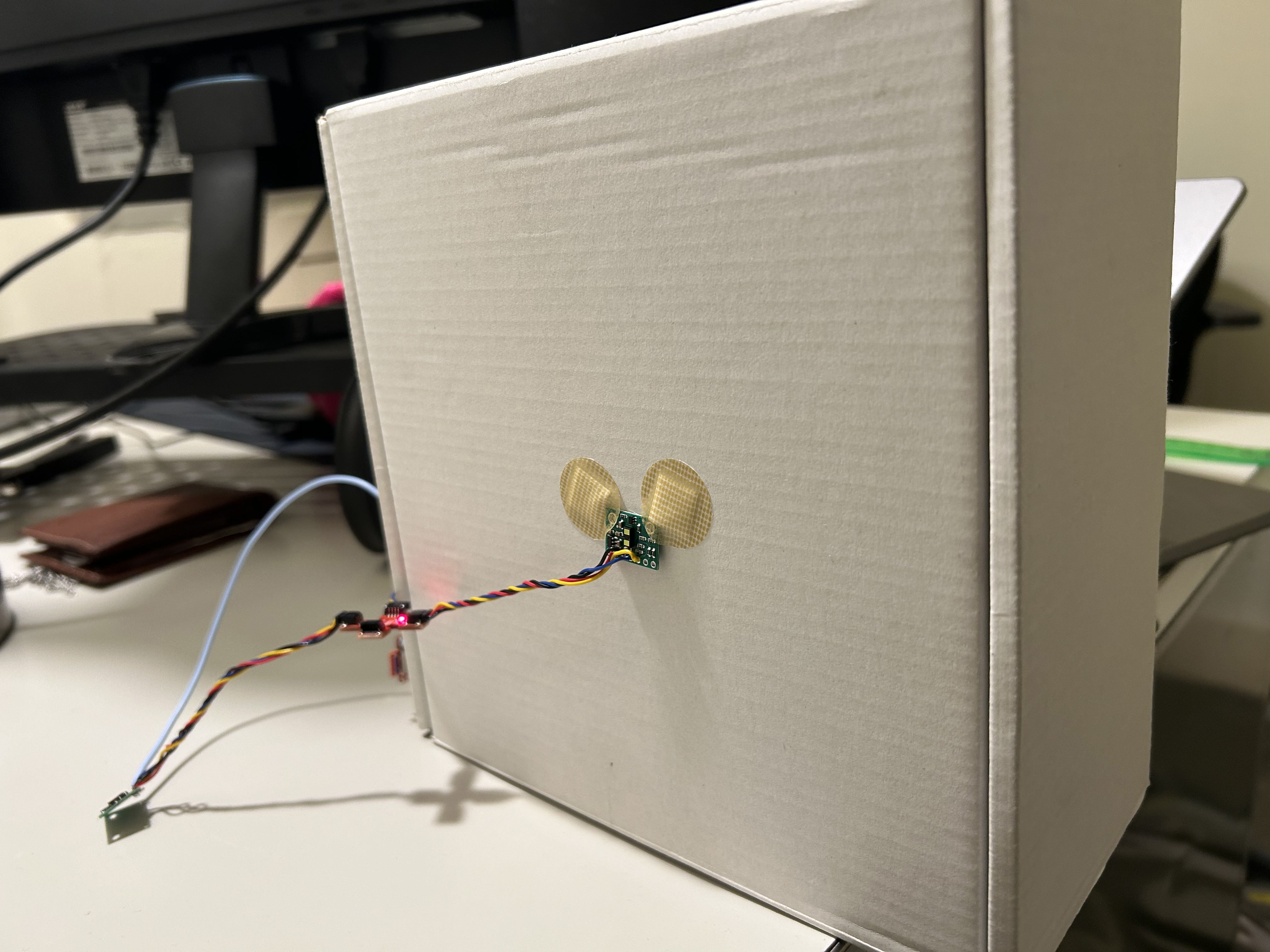
To test my cofiguration, I taped the sensor to the back of my laptop as shown below at known distances from the wall.
Then I collected the data from the sensor and sent it via bluetooth to plot the data. According to the datasheet, some accuracy, repeatability
and ranging were performed using 32 measured distances. I used the average of these distances to get the final distance.
Below is an excerpt of the code to configure the distance mode.
distance_sensor.startRanging();
distance_sensor.setDistanceModeShort();
distance_sensor.setTimingBudgetInMs(33);
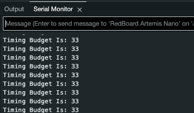
And similarly to previous labs, we can send 32 data points via bluetooth. And for good measure, I print out the timing budget
case TOF:
    for (int i = 0; i < 32; i++) {
    distance_sensor_1.startRanging();
    while (!distance_sensor_1.checkForDataReady()) {
        delay(1);
    }
    int distance = distance_sensor_1.getDistance();
    distance_sensor_1.clearInterrupt();
    distance_sensor_1.stopRanging();
    float distanceInMM = distance;

    tx_estring_value.clear();
    tx_estring_value.append(distanceInMM);
    tx_characteristic_string.writeValue(tx_estring_value.c_str());
    Serial.print("Timing Budget Is: ");
    int timing_budget = distance_sensor_1.getTimingBudgetInMs();
    Serial.println(timing_budget);
    }
 ToF Distance
The setup to test the sensors is shown below. The sensor is placed on the back of a box and put at some distance from a wall in a well lit room.
 ToF Setup
Taking a range of measurements and averaging the results over 32 data points, the following plot shows how the sensor compares to the actual measurement taking by a ruler
 ToF Accuracy
The readings don't deviate much from the ruler. The accuracy of the sensor is reliable.
To look at repeatability, I took the standard deviation of the repeated measurements and averaged them out.
sd = []
for meas in all_data:
    sd.append(np.std(meas))
print(np.mean(sd))
The result was 1.6890991200450813. This gave an average standard deviation of 0.00169m. This is an indication that the sensor is relatively stable and repeatable.
Finally, the plot shows the sensor to give consistently accurate measurements for a range of distances. However, the datasheet shows that the short distance mode will continue to give reliable results for up to 130cm. This is a good indication that the sensor is working as expected.
I used the following snippet to investigate the ranging time:
unsigned long start = millis();
distance_sensor_2.startRanging();
...
distance_sensor_2.stopRanging();
unsigned long diff = millis() - start;
The result was printed out to the serial monitor. Ranging hovered around 29ms for the short distance mode. This is a good indication that it is meeting the timing budget.
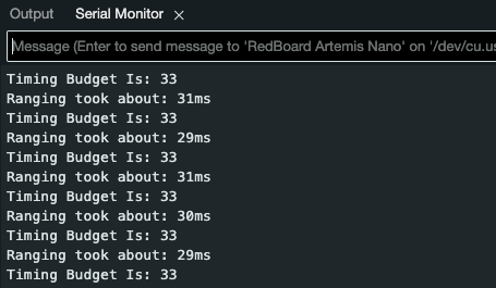 ToF Ranging
2 ToF sensors and the IMU: Discussion and screenshot/video of sensors working in parallel
To ensure both sensors are working, I used my findings from the prelab to configure one of the I2C addresses to a different address.
I first set the XSHUT pin as an output, then I set it to low to configure the address of the second sensor. Once concluded,
I set the XSHUT pin to high so the sensor 1 assumes the default address.
#define SHUTDOWN_PIN 8
#define INTERRUPT_PIN 3
SFEVL53L1X distance_sensor_1(Wire, SHUTDOWN_PIN, INTERRUPT_PIN);
SFEVL53L1X distance_sensor_2;
...

// To use two sensors
pinMode(SHUTDOWN_PIN, OUTPUT);
// XSHUT Low on sensor 1
digitalWrite(SHUTDOWN_PIN, LOW);
distance_sensor_2.setI2CAddress(0x77);
digitalWrite(SHUTDOWN_PIN, HIGH);
And following instructions from the previous lab, I was able to wire the IMU and collect it's data.
 Two ToF Sensors
Tof sensor speed
To investigate how long is was taking to get a measurement, I use a timestamp just before ranging, and at the end to see how long it took.
unsigned long start = millis();
// start ranging on both sensors

...

// stop ranging on both sensors
unsigned long ready = millis() - start;
...
// check if data is sent and processed
ready = millis() - start;
Serial.print("All done in: ");
Serial.print(ready);
The following highlights the results.
Stop Ranging at 33ms
All done in 47ms
So it took about 33ms which makes sense as I set the timing budget to 33ms for both sensors to get a measurement. And about 14 ms to convert both readings to feet and inches, and also print out the data to the serial monitor. We can speed things up by reducing the timing budget at the cost of accuracy. Or getting rid of the conversion to feet and inches and the multiple serial prints. I decided to go with the latter option.
I was able to get the following results.
Stop Ranging at 33ms
All done in 39ms
This is is signifcanly faster implementation than the previous result!
Time v Distance:
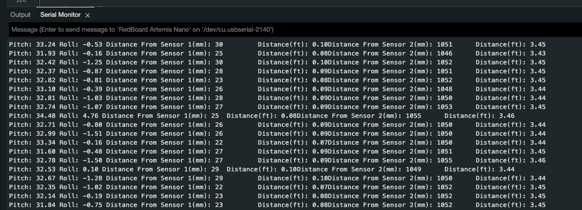
I was able to obtain a Time vs Distance plot by sending the data from the board to my laptop via bluetooth. I created a new command that allowed me to send data from both sensors and the IMU. I essentially collected data for a duration of 5 seconds and sent it via bluetooth.
unsigned long start = millis();
while (millis() - start < duration) {
    distance_sensor_1.startRanging();
    distance_sensor_2.startRanging();
    while (!distance_sensor_1.checkForDataReady()) {
    delay(1);
    }
    while (!distance_sensor_2.checkForDataReady()) {
    delay(1);
    }
    int distance = distance_sensor_1.getDistance();
    int distance2 = distance_sensor_2.getDistance();
    distance_sensor_1.clearInterrupt();
    distance_sensor_1.stopRanging();
    distance_sensor_2.clearInterrupt();
    distance_sensor_2.stopRanging();

    if (myICM->dataReady()) {
    myICM->getAGMT();
    float pitch = atan2(myICM->accY(), myICM->accZ()) * 180 / M_PI;
    float roll = atan2(myICM->accX(), myICM->accZ()) * 180 / M_PI;
    imu_pitch[data_sent] = pitch;
    imu_roll[data_sent] = roll;
    }


    tof_in_mm[data_sent] = distance;
    tof2_in_mm[data_sent] = distance2;
    times[data_sent] = millis();
    data_sent++;
}

for (int i = 0; i < data_sent; i++) {
    tx_estring_value.clear();
    tx_estring_value.append((float)times[i]);
    tx_estring_value.append(",");
    tx_estring_value.append(tof_in_mm[i]);
    tx_estring_value.append(",");
    tx_estring_value.append(tof2_in_mm[i]);

    tx_estring_value.append(",");
    tx_estring_value.append(imu_pitch[i]);
    tx_estring_value.append(",");
    tx_estring_value.append(imu_roll[i]);
    tx_characteristic_string.writeValue(tx_estring_value.c_str());
}

// Start Index over for next batch;
data_sent = 0;
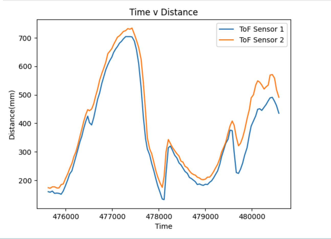 ToF Time vs Distance
Time v Angle:
And finally, I was able to obtain a Time vs Angle plot by sending the data from the board to my laptop via bluetooth using the same command as above.
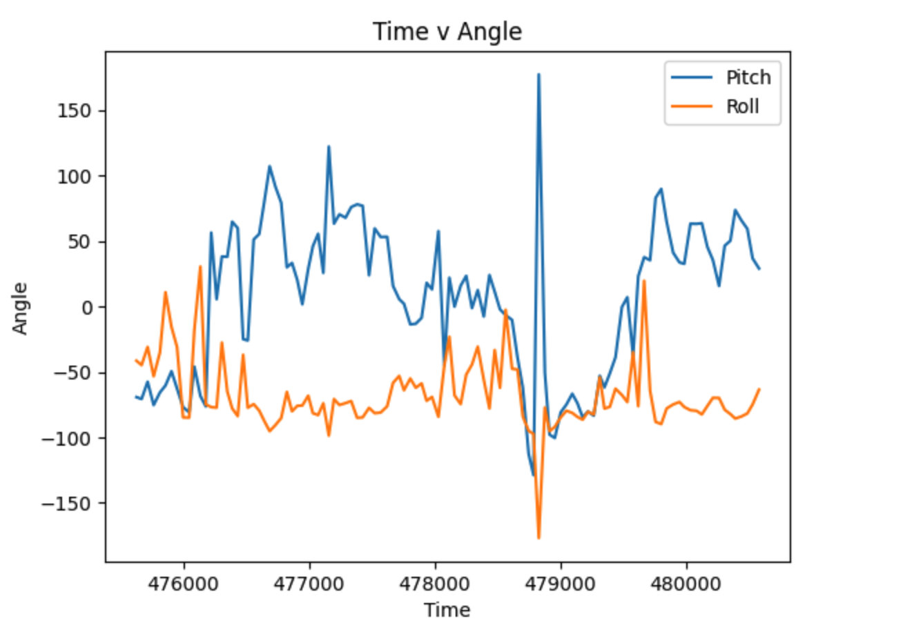 ToF Time vs Angle
Conclusion
Overall, this was a fun lab working with the VL53L1X ToF sensor. I was able to get a good understanding of the sensor's capabilities and limitations. And also enjoyed soldering wires to the sensor and the Artemis board.